Monthly Archives: November 2015

Confidence Game Creates a Dilemma for the Fed

  • As the December FOMC meeting approaches, the Fed faces a real dilemma. Does the Fed leave interest rates on hold and risk undermining market confidence in the US recovery and the Fed’s own credibility? Or does the Fed start the process of raising interest rates, a move which will put in on a path that could also severely damage economic confidence?
  • While it may be not clear to markets at this point, the view of The Money Enigma is that the Fed faces what could best be described as the “Bad Debtors’ Dilemma”. In simple terms, if you have borrowed lots of money and can’t really afford to repay it, how do you keep the faith of creditors? Do you wait as long as possible to begin repayments or do start making small repayments now in the hope that things will somehow work out?
  • The dilemma facing the Federal Reserve is does the Fed push back normalization for as long as possible hoping markets won’t notice, or do they start the process hoping that normalization will not disrupt the economy and damage market confidence?
  • Over the past ten years, the Fed has engaged in an extraordinary series of unorthodox policy actions, most notably cutting the Fed Funds rate to zero and quintupling the size of the monetary base. The success of this unorthodox policy approach has been underwritten by the notion that the US economy will recover “in time” and that the Fed will normalize monetary policy settings “eventually”.
  • However, the markets, just like the unfortunate lender to our bad debtor, won’t wait forever. If the Fed waits too long to begin the process of “normalization”, then long-term economic confidence could be damaged.
  • Alternatively, if the Fed does begin the process of normalization but then starts stalling on further rate rises or, even worse, stops the process of normalization and engages in more quantitative easing, then long-term confidence could be severely damaged. In either scenario, the end result is a poor one for the Fed and the US economy.
  • The key problem for the Fed is that long-term economic confidence underwrites the value of the US Dollar. If market confidence in the long-term economic future of the United States is damaged, then the value of the US Dollar will fall and this will trigger a marked acceleration in inflation. Any sudden rise in inflation will not only damage the Fed’s credibility but also severely limit its ability to control economic outcomes.

You can listen my interview with the MiningMaven on this article by clicking on link below.

The Bad Debtors’ Dilemma

Let’s imagine that an old friend came to visit you a few years ago and asked to borrow some money. Your friend explained to you that they had hit some tough times and you decided to lend them $3,000.

A few months later, your friend returned. Their situation had not improved and they asked for some more cash. Again, you knew this person well so you felt happy lending them another $3,000. In fact, you were so confident in your friend’s ability to repay the money eventually that you said that they could come to you again if they needed to.

Sure enough, your friend turns up again a few months later and borrows another $4,000 on top of the $6,000 that you had already loaned them. By now the debt is significant, but you feel confident that your friend will repay the debt eventually. In fact, you tell your friend that there is “no rush” to repay the debt.

Now, what happens if your friend struggles to get back on his/her feet?

Your friend knows that, at some point, you are going to want your money back. So, what should your friend do, particularly if your wallet represents their “last resort”?

Should your friend, the bad debtor, keep putting off making any repayment to you, the lender, for as long as possible and hope that you don’t begin suspecting there is a problem? Alternatively, should the bad debtor attempt to keep the lender’s confidence by starting to make a series of small repayments?

For the bad debtor, the problem presents a real dilemma. On one hand, it is tempting to make no repayment and just hope that the lender doesn’t begin to suspect that something is wrong. However, this approach is not sustainable: the lender will get suspicious eventually.

On the other hand, starting to make small repayments, for example $100 per month, can also backfire even if does buy a bit more time. For example, the lender may begin to question why the monthly repayments are so small and why larger repayments are not forthcoming.

More problematically, if the bad debtor suddenly suspends the token $100 per month repayment, then this will definitely raise suspicions. For example, imagine your friend does start repaying you $100 per month for six months but then suddenly asks to reduce the monthly payments to $50 per month. Worse still, imagine how you would feel if your friend stopped the repayments altogether and came back to you asking for more money!

The Fed’s Dilemma

While the analogy may not be perfect, the view of The Money Enigma is that the Fed faces a dilemma similar to that faced by our bad debtor.

In simple terms, the Fed is engaged in a confidence game. The key to winning this game is ensuring that markets believe that the long-term economic future of the United States is sound. So far, the Fed has been very successful in playing this game, helped by the fact that the United States has a tremendous history of economic success. However, the inevitable monetary policy tightening cycle that confronts the Fed will test this market confidence.

In terms of our Bad Debtor analogy, the implementation of ZIRP by the Fed represents the first $3,000 lent to our bad debtor. Markets were happy for the Fed to cut the Fed Funds rate to zero in 2008 because there was a financial crisis and the Fed had a long and successful history of lowering interest rates in a time of crisis.

However, ZIRP was not enough to resolve the crisis. Therefore the Fed quickly came back to markets for the next $3,000, i.e. QE1. Although quantitative easing represented an unorthodox policy approach, market confidence was not damaged because this sudden expansion of the monetary base was viewed as being “temporary” in nature.

Ultimately, the Fed perceived that QE1 was insufficient, so the Fed came back for the next $4,000: QE2 and QE3.

Despite these extraordinary policy measures, the markets have never lost faith in the Fed. The view of the markets has been and remains today that the US economy will continue to do well over time and that this will allow the Fed to “normalize” monetary policy eventually.

The problem is that we are now approaching the point where this confidence will be tested. At some point, the Fed must normalize policy just as the bad debtor must repay the debt.

The challenge for the Fed is figuring out a way to do this that doesn’t damage market confidence. If the Fed is too slow to normalize policy, the markets may begin to lose faith in the Fed. If the Fed is too aggressive in its attempts to normalize policy, then it could easily knock the economy back into recession.

The “middle road” also represents a potential problem for the Fed. For example, let’s imagine that the Fed does raise the Fed Funds rate by 150 basis points over the next 12 months without damaging the economy. Superficially, this would be a great outcome. However, it still leaves a problem. The Fed still needs to reduce the monetary base by at least $2 trillion. In essence, raising short-term rates is only repaying the first $3,000. Ultimately the Fed needs to repay the entire $10,000 to keep the faith of the markets, i.e. it must raise short-term rates and reduce the monetary base to pre-crisis trend levels.

The greater concern is what happens if the Fed begins the normalization process in December but then has to stall this process or reverse it?

For example, what happens to market confidence in the long-term future of the United States if the Fed does raise interest rates to 0.75% and the US economy falls into recession in mid 2016? Alternatively, what happens to confidence if the Fed decides to sell $1 trillion of the bonds on its balance sheet and this triggers a crash in global equity and bond markets? [This second scenario is something that has been discussed in a previous post titled “Has the Fed Created the Conditions for a Market Crash?”]

In many ways, it is easier for the Fed to sit on its hands and do nothing rather than tempt these outcomes, just as it is easier for our bad debtor to avoid showing his/her hand by starting the repayment process. But ultimately, the misadventures of the Fed need to be reversed and this will be the point at which the confidence of the markets will be tested.

Why Does Long-Term Economic Confidence Matter?

Just as our bad debtor needs to maintain the confidence of our lender, so the Fed needs to maintain the confidence of markets. More specifically, the Fed needs to ensure that markets do not lost their faith in the long-term economic future of the United States.

Why does confidence in the future of the economy matter? Well, there are a couple of key reasons.

First, and most obviously, a loss of faith in the future of the United States is bad for business. If markets start to believe that the long-term rate of economic growth in the US will be much lower than previously expected, then capital spending will be slashed, business formation will be delayed and jobs will be lost.

Second, and less obviously, confidence in the long-term economic future of our society is a key determinant of the rate of inflation. In simple terms, high levels of confidence support the value of the dollar and keep a lid on the rate of inflation. Conversely, a sudden decline in long-term confidence could lead to a collapse in the value of the dollar and a sudden rise in prices.

The reasons for this are complicated, but we can use our bad debtor analogy to help explain the point.

Think back to our earlier example. Why does our bad debtor want to keep his/her financial situation a secret? In simple terms, our bad debtor knows that if the lender’s confidence is lost, then the lender will want his/her money back and will not be inclined to lend our debtor any more money.

In more technical terms, we can say that our debtor wants to prevent his/her cost of debt capital from rising. If the lender loses confidence in our debtor, then the lender will probably require a higher rate of interest on existing and future monies lent to that debtor.

The Fed faces a similar challenge, although it is a concept that is poorly understood by most economists. In essence, when the Fed expands the monetary base (“prints money”), it creates claims against the future output of society. In this sense, the monetary base can be considered to be the “equity of society”.

While confidence in the long-term economic future of society remains high, the Fed can issue money without impacting its cost of equity, i.e. without debasing the value of the US Dollar. However, if long-term confidence is lost, then the Fed’s “cost of equity” will rise. In other words, the Fed can continue to issue more dollars, but the value of each dollar is less.

How does a decline in the value of the dollar show up in the real world? Inflation.

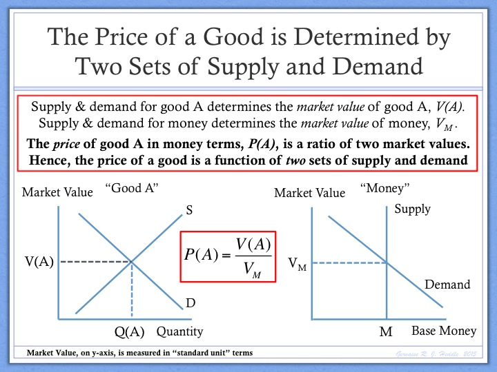
All else remaining equal, if every dollar is worth less in absolute terms, then the price of all goods in dollar terms must rise. Every price is a relative measurement of the market value of two items. More specifically, the price of one good, the “primary good”, in terms of another good, the “measurement good”, is a relative measure of the value of the primary good in terms of the measurement good. If the market value of the measurement good falls, then the price of the primary good in measurement good terms will rise.

Therefore, if the value of money falls, then prices as expressed in money terms will rise and the rate of inflation will accelerate.

In summary, the view of The Money Enigma is that the Fed must maintain the confidence of the market just as our debtor must maintain the confidence of the lender. If the Fed loses the confidence of the market, then the Fed’s cost of capital will rise, just as the debtors cost of capital will rise if it loses the faith of its creditors. In practical terms, a rise in the Fed’s “cost of capital” means that the value of the US Dollar will fall, inflation will accelerate and the Fed will largely lose the ability to manage macroeconomic outcomes.

If you are interested in reading more about why the value of fiat money is so heavily dependent upon long-term economic confidence, then I would encourage you to read the following posts. First, I would suggest reading “The Evolution of Money: Why Does Fiat Money Have Value?” which attempts to explain why paper money with no intrinsic worth has any value at all. Second, I would suggest reading the follow on article “What Factors Influence the Value of Fiat Money?” If you are interested in the notion that the monetary base is, in essence, an equity instrument and proportional claim in the future output of society, then I would encourage you to read an older post “Money as the Equity of Society”.

Does Excess Demand Cause Inflation?

  • The view of most economists is that the key driver of inflation is the strength of the economy. If monetary policy is too accommodative, then it can create too much demand and the economy can “overheat”, leading to higher rates of inflation. Conversely, if the economy weakens, then deflation, not inflation, becomes the key risk.
  • This quintessentially Keynesian view of the world has been drummed into the minds of market participants by a succession of Fed officials, nearly all of whom have argued that the key role of the Fed is too ensure that the temperature of the economy remains “just right”, i.e. not too hot and not too cold.
  • But does the strength of the economy really matter to inflation? Is “too much demand” the primary cause of inflation? And is it a given that a weak economy must result in deflation?
  • The view of The Money Enigma is that excess demand is not the primary cause of inflation. Rather, the primary cause of rising prices over time is a fall in the value of money. While swings in the economic cycle may somewhat abate or accentuate an inflationary trend, the underlying trend is always determined by the value of money, not the value of goods.

When Did “Too Much Demand” Create Inflation?

If you listened only to Fed officials, then you might quickly come to the view that the rate of inflation is primarily a function of the strength of the economy: a strong economy produces higher levels of inflation and a weak economy produces low levels of inflation or even deflation. This is the prevailing view that is implicit in the thought process of most talking heads on CNBC and that appears in nearly every debate regarding the outlook for inflation.

However, the historical evidence for this proposition is thin.

While there have been numerous academic studies conducted on this issue, I’d like to encourage readers to step back from a moment and consider this question for themselves: “When did too much demand create inflation?”

What specific periods of history can you point to, either in the United States or any other country, where high levels of inflation have clearly been created by too much aggregate demand?

There are two ways you can approach this question. Either you can look at periods of high inflation and try to make some judgment about whether there was “too much demand” at the time, or you can look at periods of economic strength and see what happened to inflation during those periods.

While everyone will have a slightly different interpretation of history, the view of The Money Enigma is that it is very difficult to find any clear correlation between economic strength and inflation.

At the most basic level, it is well known that episodes of high levels of inflation, i.e. hyperinflation, have most commonly been associated with very weak economic conditions.

For example, one could hardly claim that hyperinflation in Zimbabwe in the 1990-2010 period was caused by “too much demand”! Similarly, one could hardly claim that prices are rising in Venezuela because Venezuela is the poster child of economic success!

Putting the issue of hyperinflation to one side, it is still very difficult to find clear anecdotal examples where economic strength created to inflation.

For example, the late 1990s was one of the strongest economic periods in US history. During the late 1990s, unemployment was low, consumer spending was high and capital spending, particular on technology, was off the charts.

So, what happened to inflation in the US during the late 1990s? It fell. Inflation fell from 3% in 1995 to sub 2% by 1997-98 and only staged a recovery back to the 3% rate in the last part of 1999 when the participation rate jumped to a record high. In this example, a stronger economy actually seemed to lead to a low inflationary trend, with a small cyclical bump in inflation right at the point that the economy was blowing steam.

Conversely, we can think of the stagflation in the 1970s. In the 1970s, inflation rose from a 5% annual rate and peak at nearly 15%. This peak in the rate of inflation in 1979-1980 was not marked by “good economic times” but rather an economy operating at stall speed.

Clearly, this type of anecdotal evidence does not supply us with a scientific analysis of the issue. However, many academic studies of this issue have been undertaken and the results are, at best, inconclusive.

In technical terms, the notion that “too much demand creates inflation” is known as the Phillips Curve. The Phillips Curve is a core part of New Keynesian thought and the current economic orthodoxy practiced by the major central banks. In essence, the Phillips Curve states that there is an inverse relationship between the rate of unemployment and the rate of inflation. Stated simply, as the economy approaches full employment, wages and prices must rise.

John Hussman, fund manager and economist, provides an excellent critique of the Phillips Curve and the empirical evidence supporting it in his post “Will the Real Phillips Curve Please Stand Up?”

In simple terms, Hussman’s point is that if there is a strong inverse correlation between unemployment and inflation, then that should show up on a chart plotting unemployment against inflation. It doesn’t. Economists have tried to prove the relationship by adjusting the models, but even then the relationship between unemployment and inflation remains elusive.

One Price, Two Values

If the notion that “excess demand causes inflation” is not supported by empirical evidence, then why do so many economists cling to the idea? Why do market commentators persist with the fable that a “strong economy” equals inflation and a “weak economy” equals deflation?

Part of the reason for the persistence of this myth is that it is easy to communicate. Most people understand the basic microeconomic concept that, all else remaining equal, more demand for a good leads to a higher price for that good. Therefore, it is easy for people to extrapolate this idea from one good to many: if there is more demand for all goods, then the price of all goods should rise.

The problem is that, at a macroeconomic level, the forces of price determination are far more complex than this and one simply can’t carry-forward the set of microeconomic assumptions that are associated with basic supply and demand analysis.

At a more fundamental level, the problem with the basic supply and demand analysis described above and presented in most economics textbooks is that provides a partial, one-sided and incomplete view of the microeconomic price determination process.

The view of The Money Enigma is that every price is a relative measurement of the market value of two goods. For example, the price of apples in terms of money is a relative expression of both the market value of apples and the market value of money. The price of apples in money terms can rise for one of two reasons: either (a) the market value of apples rises or (b) the market value of money falls.

Most people believe that “price” and “market value” are synonymous, i.e. they mean the same thing. The view of The Money Enigma is that they are very different. “Market value” is a property possessed by economic goods. “Price”, on the other hand, is merely one method of measuring this property. More specifically, price is a relative measurement of the property of market value: a price measures the market value of one good in terms of another good.

In mathematical terms, we can say that the price of a good is a ratio of two market values, where each of those market values are measured in “absolute terms”, i.e. in terms of a “standard unit” of measurement. [The measurement of market value is a complicated but important topic and I would highly encourage you to read a recent post on this issue titled “The Measurement of Market Value: Absolute, Relative and Real”.]

Price as Ratio of Two Market Values

If this basic theory is correct, then it suggests that every price is determined by not one, but two sets of supply and demand. Supply and demand for apples determines the market value of apples. Supply and demand for money (the monetary base) determines the market value of money. The price of apples in money terms is determined by the ratio of these two market values.

Price Determined by Two Sets Supply and Demand

Now, why is this microeconomic theory relevant to our discussion regarding the relationship between excess demand and inflation? Well, this microeconomic theory of price determination can be extended to a macroeconomic theory of price level determination.

If every price is a relative measurement of the market value, then the price level itself is also a relative measurement of market value. More specifically, the price level measures the market value of the basket of goods in terms of the market value of money. In this sense, the price level can be considered to be a ratio of two market values. [See “Ratio Theory of the Price Level” for a more detailed discussion].

Ratio Theory of the Price Level

Ratio Theory implies that the price level can rise for one of two reasons. Either (a) the market value of the basket of goods rises, or (b) the market value of money falls. In other words, either the numerator in the equation above rises or the denominator falls.

The problem with most commentary regarding the outlook for inflation is that it implicitly focuses only on the numerator in our price level equation.

Shifts in aggregate demand and supply for goods and services can certainly impact the market value of these goods and services. Moreover, an economy that is “overheating” may well experience a temporary rise in the market value of goods.

Goods Money Framework

However, while these are important factors in near-term price level determination, the view of The Money Enigma is that they are primarily cyclical factors and do not explain changes in the inflationary trend. For example, “too much demand” can’t explain why the inflationary trend rose in the 1970s, or why it fell in the 1990s, or why Zimbabwe experienced hyperinflation in the 2000s.

The Value of Money and Inflation

If changes in the numerator, the “market value of basket of goods”, can not explain major shifts in the underlying inflationary trend, then clearly there is only one other factor that can explain these shifts: the denominator in our equation, the “market value of money”.

The view of The Money Enigma is that excess demand is not the primary driver of the long-term trend in inflation. Rather, the primary driver of rising prices as measured over long periods of time is a fall in the value of money.

In terms of our price level equation, swings in the economic cycle will impact the value of goods (the numerator in our equation) and this may somewhat abate or accentuate an inflationary trend. However, the underlying trend is always determined by changes in the value of money (the denominator in our equation).

The “value of money” is a concept that most economists struggle with. The reasons for this are complex and are discussed in a recent post “The Value of Money: Is Economics Missing a Variable?”

In essence, the problem relates to one of measurement. The “value of money” is generally measured in relative terms: for example, the “purchasing power of money” measures the value of money in terms of the value of goods (it is, after all, simply the reciprocal of the price level). However, in order to isolate the “value of money” as its own independent variable, one must measure the value of money in absolute terms, i.e. in terms of a “standard unit” for the measurement of market value.

If this all sounds a bit too technical, then think of it this way. The money in your pocket has value. If it didn’t you wouldn’t accept it in exchange and others wouldn’t accept in exchange. The value of money goes up and down. Moreover, it goes and down independently of the value of other goods, such as apples, and it does up and down independently of the value of the basket of goods.

If the value of money declines significantly over a period of time, then, all else remaining equal, the price of other goods in money terms will rise. Why? Well, if each unit of money becomes less valuable, then people will ask for more units of money for each apple sold or each hour worked.

The view of The Money Enigma is that major shifts in the price level and the inflationary trend are driven by changes in the value of money and the rate of depreciation of the value money respectively.

For example, the price level in the United States has risen roughly tenfold since the 1950s. Does it seem more likely that this tenfold increase in prices has been driven by (a) an excess of aggregate demand for most of the last fifty years, or (b) a decline in the value of the US Dollar due to growth in the monetary base that has dramatically exceeded real output growth?

Frankly, (a) is implausible. The US economy has experienced many periods of slack and weakness over that time that could have easily unwound any temporary inflationary pressures due to “too much demand”. In contrast, (b) is entirely plausible, particularly if one believes that money is a claim on the output of society and that the value of money depends primarily upon the growth of real output relative to the monetary base.

In summary, the view of The Money Enigma is that excess demand can, at least temporarily, lead to an acceleration of inflation. However, in most cases, the impact is likely to be short-lived and is largely irrelevant to the underlying inflationary trend that should concern policymakers.

The primary driver of the core inflationary trend is not excess demand, but rather the decline in the value of money that results when policymakers grow the monetary base at a rate that exceeds the growth in real output.

Will the Velocity of Money Increase in 2016?

  • Over the past eight years, the velocity of money has collapsed. Since its peak in 2007, the velocity of narrow money seems to have fallen off a sheer vertical cliff, as illustrated in the chart below. However, over the past year or so, there are early signs that the velocity of money has stabilized, albeit at exceptionally low levels.
  • Does this stabilization mark a turning point for the velocity of money? Has the velocity of money reached its nadir? And what factors might drive the velocity of money higher in 2016 and beyond?
  • The view of The Money Enigma is that the velocity of money has probably reached its low point. More specifically, there are three possible factors that could drive the velocity of money higher in 2016.
  • First, the US economy could reaccelerate, requiring a higher turnover of money to facilitate the extra transactions in the economy.
  • Second, the Federal Reserve could begin to reduce the monetary base. All else remaining equal, if there is less money in the system, then the money that remains needs to turn over more often to “get the job” done, i.e. to facilitate the same monetary value of economic transactions.
  • Third, the value of money could decline. All else remaining equal, if each unit of money (each dollar) becomes “less valuable” in an absolute sense, then each unit of money must change hands more times in order to complete the same “absolute value” of economic transactions.
  • The view of The Money Enigma is that the velocity of money is close to its nadir. Why? Well, either the Fed will significantly reduce the monetary base, leading to an almost mathematically certain rise in the velocity of narrow money, or the Fed’s inaction will cause a significant decline in the value of money and a concomitant rise in the velocity of money.
  • The relationship between the velocity of money and the “value of money” is poorly articulated by mainstream economics. In order to fully explain this idea, we will discuss a new model for the velocity of money and focus on the relationship between each of the three factors described above and the velocity of money. More specifically, we will explore the critical relationship between the value of money and the velocity of money.

A Brief Overview

Since 2007, the velocity of narrow money has collapsed. The chart immediately below illustrates how the velocity of M1 has fallen sharply over the past eight years.

velocity of money M1

In the last 12 months, the velocity of money seems to have stabilized at exceptionally low levels, levels that have not been seen since the early-mid 1970s. Interestingly, the chart above does seem to suggest that the velocity of money tends to fluctuate within a wide band. Indeed, many economists still believe that the velocity of money tends to “revert to the mean” over long periods of time. So, will the velocity of money begin to revert to the mean in 2016? And if it does, what are the implications for inflation?

In order to understand what might drive the velocity of money higher in 2016 and beyond, we need to do two things.

First, we need to derive a model of the velocity of money that is “useful”, not just a rearrangement of the famous equation of exchange. The view of The Money Enigma is that a useful model for the velocity of money must incorporate an explicit role for the “value of money”.

Second, we need to review the experience on the last eight years in terms of this model. In this week’s post, it will be argued that the reason the velocity of money declined so sharply over the past eight years is because the massive expansion in the monetary base did not trigger a concomitant fall in the value of money.

Once we complete these two steps, then we will apply our model to the outlook for 2016. The view of The Money Enigma is that there are, as always, three key factors that could drive the velocity of money higher. But, in practice, only one or two of these factors are likely to drive a sharp rise in the velocity of money over the next few years.

A Model for the Velocity of Money

In this section, we are going to explore how the model for the velocity of money below is derived and, more importantly, what it means.

Velocity of Money Model

There are two key terms in the model above that will be unfamiliar to new readers. The first is the “market value of the basket of goods”, denoted “VG. The second is the “market value of money”, denoted “VM. In both cases, the property of market value is measured in terms of a “standard unit”. I shall explain what this means in a moment.

At a high level, the model for the velocity of money above suggests that the value of money, “VM, plays a critical role in the determination of the velocity of money. All else remaining, as the value of money falls, the velocity of money rises.

The view of The Money Enigma is that the standard equation for the velocity of money (v=pq/M) is not a useful predictive or explanatory model. Simply rearranging the equation of exchange to put the velocity of money on the left hand side and nominal output divided by money supply on the right hand side tells us very little about what actually drives the velocity of money.

More specifically, if a model for the velocity of money is to be useful at explaining why the velocity of money can rise and fall so sharply, then it must incorporate an explicit role for “the variable that economics forgot”, the “value of money”.

However, in order to incorporate the value of money in our model for the velocity of money we must first isolate the value of money as an independent variable.

Isolating the value of money as an independent or “standalone” variable is something that mainstream economics has consistently failed to achieve. The reasons for this are complex and are discussed at length in a recent post titled “The Value of Money: Is Economics Missing a Variable?”

In essence, the problem relates to how economics measures the property of “market value” or what others might refer to as “value in exchange”. In order to isolate the value of money as an independent variable, we must measure the market value of money in absolute terms, not relative terms. Moreover, we can only measure this property in absolute terms if we adopt a “standard unit” for the measurement of market value.

While most people think of “market value” and “price” as synonymous, the view of The Money Enigma is that “market value” and “price” are not the same thing. Rather, price is merely one method of measuring the property of market value.

Market value is a property that all economic goods possess. For example, an apple has market value and, in order to acquire an apple from you, I must offer you something valuable in exchange. The market value of that apple will fluctuate, completely independent of changes in the market value of any other good.

The price of a good is a relative measure of the market value of one good in terms of the market value of another. For example, if an apple is twice as valuable than a banana, then the price of apples in banana terms is two bananas. Moreover, the price of apples in banana terms can rise for one of two reasons: either, (a) apples become more valuable, or (b) bananas become less valuable.

The point is that “market value” is a property and “price” is a relative measure of this property. This observation leads us to our next question: if market value can be measured in relative terms, then can it be measured in absolute terms?

The simple answer is “yes”. However, in order to measure any property in absolute terms, one must adopt a “standard unit” for the measurement of that property. A “standard unit of measurement” is a theoretical unit of measure that is invariable in the property being measured. While no good is invariable in the property of market value, we can create a theoretical good that is invariable in that property and use this as our standard unit.

Now, how does all this relate to the “value of money”?

Typically, economics measure the “value of money” in relative terms. Most commonly, the value of money is measured in terms of the value of the basket of goods. This is known as the “purchasing power of money” and is simply the inverse of the price level.

The problem with measuring the value of money in this way is that it doesn’t allow us to isolate the value of money as an independent variable. For example, if the purchasing power of money falls, then we don’t whether it was because (a) the value of money fell, or (b) the value of the basket of goods rose.

However, if we adopt a standard unit for the measurement of market value, then, at least theoretically, we can isolate the value of money and the value of the basket of goods as two separate variables and analyze them separately.

Moreover, we can extend our observation that “every price is a relative expression of market value” to the price level. If every price is a relative measure of market value, then the price level is also a relative measure of market value. More specifically, the price level is a relative measure of the value of the basket of goods in terms of the value of money.

Mathematically, we can express the price level as a ratio of two values, an idea that was discussed at length in a recent post titled “Ratio Theory of the Price Level”. In simple terms, if we denote the market value of the basket of goods as measured in terms of the standard unit as “VG and we denote the market value of money as measured in terms of the standard unit as “VM, then the price level is simply the first term divided by the second term.

Ratio Theory of the Price Level

What does Ratio Theory imply? In simple terms, Ratio Theory states that the price level can rise for one of two reasons: either (a) the value of the basket of goods rises, or (b) the value of money falls.

Now, let’s return to our discussion of the velocity of money. How can Ratio Theory help us understand the possible drivers of the velocity of money?

The great advantage of Ratio Theory, in regards to this discussion, is that it allows us to substitute out the price level “p” in the equation of exchange and replace it with the two variables described above.

Derivation of Velocity of Money Model

Suddenly, we have a new model for the velocity of money that can provide us with some useful and rather intuitive insights into what really drives the velocity of money. More specifically, we have a model for the velocity of money that contemplates an explicit role for the “value of money”: all else remaining equal, as the value of money falls, the velocity of money rises.

Now, let’s take this model for the velocity of money and think about what has happened over the past eight years.

Why Has the Velocity of Money Collapsed?

Let’s take our new model for the velocity of money and think about why the velocity of money may have collapsed over the past eight years.

Velocity of Money Model

From a theoretical perspective, there are four variables that could drive a decline in velocity. However, in practice, the two variables in the numerator tend to be relatively stable. Rather, most of the major variations in the velocity of money occur because of changes in the two variables in the denominator.

The view of The Money Enigma is that the value of the basket of goods VG and real output q are both relatively stable macroeconomic variables in principle and, over the past eight years, are unlikely to have contributed to the major decline in velocity.

Over the past eight years, real output has increased, albeit marginally, and this growth in real output has not contributed to the decline in velocity. It is possible that the value of goods, as measured in absolute terms, has declined slightly over the past eight years driven by globalization and excess supply, particularly in commodities. However, it is unlikely that a decline in the market value of goods can explain the steep drop in the velocity of money that we have seen over the past eight years.

Therefore, we need to focus on the two variables in the denominator of our model. Clearly, the large increase in the monetary base could easily explain the decline in the velocity of money. All else remaining equal, as more money is injected into the system, each unit of money needs to change hands fewer times in order to complete the same value of transaction.

But what about the second variable: the value of money? Could a rise in the value of money explain the decline in velocity?

Frankly, this seems very unlikely. Rather, it is much more likely that the value of money was relatively stable over the past eight years, a phenomenon that was reflected in the relative stability of the price level over that same period.

It is worth remembering that when the Fed first introduced quantitative easing, there were many market commentators who argued that such an expansion of the monetary base would lead to a rise in inflation. However, in practice, this didn’t occur. Rather, the price level remained relatively stable and the velocity of money collapsed. So, what happened? Why didn’t prices rise sharply when the Fed expanded the monetary base and why did the velocity of money collapse?

There is a simple answer to this question: the expansion of the monetary base didn’t trigger a collapse in the value of money. With no collapse in the value of money there was no rise in prices and, as the monetary base expanded, the velocity of money had to fall.

If the value of money had fallen, then prices would have risen and the velocity of money may have remained relatively stable. But this didn’t happen. Indeed, without a decline in the value of money over the past eight years, every injection of new money led to a further decline in the velocity of money.

The Outlook for the Velocity of Money

While predictions regarding major economic variables are notoriously unreliable, attempting to forecast the velocity of money is particularly difficult because of the wide range of factors involved. Nevertheless, let’s take another look at our model and think about what might happen to the velocity of money in 2016 and beyond.

Velocity of Money Model

The first factor that could drive an increase in the velocity of money in 2016 is a reacceleration in broader economic activity (higher VG and q). Frankly, this seems unlikely given the bias of the Fed towards tightening monetary policy, but it is possible. However, even if the US economy does accelerate in 2016, the magnitude of the shift in our numerator is unlikely to lead to a significant rise in the velocity of money.

The second factor that could drive an increase in the velocity of money in 2016 is a major reduction in the monetary base by the Federal Reserve. Once again, this seems unlikely. Even if we accept the consensus forecast that the Fed will raise short-term interest rates in 2016, any major reduction in the monetary base is unlikely given the current planning of the Fed.

If there is a major rise in the velocity of money in 2016, then it is most likely to be caused by the third and final factor: a significant decline in the value of money.

All else remaining equal, a rapid and marked decline in the value of money would have two effects. First, the price level would rise: as money becomes less valuable in absolute terms, the basket of goods becomes “more valuable” in relative terms. Second, a decline in the value of money, all else remaining equal, must lead to an increase in the velocity of money. Why? Well, thinking in absolute terms, if money becomes less valuable, then each unit of money must change hands more times to complete the same total value of economic transactions.

The obvious question that needs to be asked is why would the value of money suddenly decline in 2016? After all, the value of money has been relatively stable for the past eight years despite a fivefold increase in the monetary base.

The view of The Money Enigma is that most major fiat currencies have held their value relatively well over the past eight years because most market participants view the current experiment with quantitative easing as “temporary” in nature. In other words, most people believe that quantitative easing will be reversed in due course and that the balance sheets of the central banks will be restored to more normal levels.

The concern that has been expressed here many times is that the “temporary” flirtation with monetary base expansion will turn into a more “permanent” exercise. At the point the markets realize this is the case, the value of the major fiat currencies could decline significantly leading to a rapid rise in inflation in those countries and, all else equal, a surge in the velocity of money.

Those readers who are interested in exploring this issue further might like to read “Monetary Base Expansion: The Seven Stages of Addiction”, “The Case for Unwinding QE” and “What Factors Influence the Value of Fiat Money”.

In summary, the view of The Money Enigma is that the velocity of money has probably reached its nadir. If the Fed surprises the market and does significantly reduce the monetary base, then it is almost a mathematical certainty that the velocity of money will increase. In contrast, if the Fed fails to reduce the monetary base over the course of the next few years, then the value of money is likely to decline sharply leading to both a rise in the rate of inflation and an increase in the velocity of money.

Does the National Debt Impact the Value of the Dollar?

  • What is the relationship between a nation’s public debt and the value of the fiat currency issued by that nation? Historical evidence would suggest that high levels of government debt can trigger a sudden collapse in the value of fiat money. However, government debt levels have risen rapidly in many developed nations over the past twenty years with seemingly little impact on the value of those currencies.
  • So, what is the relationship between the national debt of the United States and the value of the US Dollar and how much debt is “too much”?
  • The view of The Money Enigma is that national debt plays a critical, but complex, role in determining the value of the dollar. More specifically, it is not “national debt” per se, but rather the market’s perception of the nation’s overall “fiscal sustainability” that directly impacts the market value of the fiat currency issued by that nation.
  • Why does “fiscal sustainability” matter to the value of fiat money? In simple terms, the government has only two choices when it decides how to fund its deficits: it can issue debt or it can expand the monetary base.
  • At the point that the market decides that the fiscal path of the nation is unsustainable and that the ability of the government to issue more debt will become increasingly restricted, the market will begin to discount the likely eventuality that both (a) real output growth will slow as taxes are raised and spending is cut, and (b) monetary base growth will accelerate as deficits need to be financed, at least partially, by more money creation.
  • This combined shift in expectations, lower output growth plus higher monetary base growth, puts downward pressure on the value of the dollar and upward pressure on the price level.
  • Why does the value of money depend upon expectations regarding the long-term future of real output and the monetary base? The value of money is sensitive to these expectations because fiat money is a financial instrument that derives it value from an implied social contract. More specifically, fiat money represents a proportional claim on the future output of society.

How Much Debt is “Too Much”?

The question “how much government debt is too much?” is an important one both for economists and policy makers. Not surprisingly, many attempts have been made to quantify the threshold at which government debt becomes dangerous.

However, attempting to provide this type of quantitative assessment is much more difficult than it first may appear. For example, Carmen Reinhart and Kenneth Rogoff in their book “This Time is Different” (2009) conducted an expansive empirical analysis of this issue covering sixty-six countries over nearly eight centuries. Their results were unable to uncover any “magic number” that can be used a threshold. Rather, the results of their work suggest that the threshold is highly variable and depends on a number of factors including the nature of the debt, the stage of the nation’s economic development and the nation’s history of default.

The issue is further complicated by the fact that, over the past twenty years, most major Western nations have accumulated levels of national debt that are exceedingly high by historical standards. Indeed, any attempt to have a sensible discussion regarding national debt is inevitability high-jacked by those that point to Japan’s record debt to GDP ratio (Japan’s national debt represents roughly 300% of its GDP) as evidence that there is no limit as to how much national debt and advanced economy can carry.

The view of The Money Enigma is that rather than focusing on quantitative thresholds, a more productive approach may involve taking a step back to think about national debt in the broad context of “fiscal sustainability” and the impact of perceived fiscal sustainability on expectations regarding the long-term economic prospects of society.

In this regard, it is helpful to put aside the specific issue of “how much government debt is too much?” and attempt to answer the more general question “how much debt is too much?”

Clearly, there is no simple answer to this question. From a corporate perspective, a sustainable level of debt will depend upon many factors including variability of cash flows, earnings growth expectations and, ultimately, some type of qualitative assessment regarding the strength of the business franchise itself.

The key point is that it is not the level of debt per se that matters, but rather perceptions regarding the sustainability of that debt. If the market suddenly decides that a given level of debt is no longer sustainable, then that is the point that the cost of both debt and equity capital can rise dramatically.

It is worth noting that, in practice, this tipping point in expectations is seldom triggered by a new issuance of debt. Rather, this tipping point most commonly occurs because of sudden change in perceptions reading the economic future of the issuing corporation.

Similarly, at a national level, the question is one of market perception regarding whether projected levels of national debt are sustainable. As the results of Reinhart and Rogoff’s work suggests, every country will differ in this regard. A national debt load that is dangerous for a commodity-focused developing nation with a history of default could represent a perfectly sustainable burden for a developed nation with a diverse and stable economy.

Moreover, as corporate experience would suggest, it is unlikely that any increase in national debt from say 100% to 120% of GDP is, in and of itself, likely to tip the balance of expectations from “sustainable” to “unsustainable”. Rather, it is more likely that a sudden loss in confidence regarding the sustainability of the US fiscal path will be triggered by other economic events such as the outbreak of war or a sudden and severe recession.

Whatever the cause of this sudden shift in perceptions, a loss of confidence in the fiscal sustainability of a nation should have dire consequences for the ability of that nation to finance its deficits. All else remaining equal, the cost of debt financing, i.e. the interest rate on government debt, will rise significantly.

Frankly, this much should be obvious. What is less obvious is how this sudden shift in perceptions impacts the value of fiat money.

The view of The Money Enigma is that fiat money is, in essence, the equity of society. Fiat money is a form of equity finance for a nation just as shares of common stock are a form of equity finance for a corporation.

If there is a sudden loss in confidence regarding the fiscal sustainability of a nation, then this impacts both the cost of debt, i.e. the interest rate on government debt, and the cost of equity, i.e. the value at which new money can be issued.

More specifically, if the market suddenly decides that the fiscal path of a nation is no longer sustainable, then the value of the fiat currency issued by that nation will decline. Moreover, this decline in the value of fiat money will be reflected in both foreign exchange rates and the domestic price level.

What Determines the Value of the Dollar?

In order to understand why the market’s assessment of fiscal sustainability matters to the value of money, we need to step back and think about what factors determine the value of fiat money and, more fundamentally, why fiat money has any value at all.

The question “why does fiat money have value?” is one that we have discussed in several recent posts including “Why Does Money Exist? Why Does Money Have Value?” and “The Evolution of Money: Why Does Fiat Money Have Value?”

At the most basic level, the view of The Money Enigma is that assets can only derive their value in two ways. Every asset is either a real asset or a financial instrument. Real assets derive their value from the physical properties. In contrast, financial instruments derive their value from the contractual properties. Moreover, a financial instrument is only an asset to one party because it represents a liability to another party.

Fiat money is a financial instrument. More specifically, fiat money derives its value from an implied contract, or “social contract”, that exists between the holders of money and the issuer of money. In essence, fiat money only has value to us because we recognize that, from an economic perspective, it is a liability of society.

The Money Enigma takes this concept further by thinking about the exact nature of the liability that fiat money represents (see “Theory of Money” section).

The view of The Money Enigma is that fiat money represents a claim on the future output of society. More specifically, fiat money represents a variable entitlement or “proportional claim” on the future output of society, much as a share of common stock represents a proportional claim on the future cash flows of a business.

The key practical implication of this theory of money is that the value of fiat money is positively correlated to expectations regarding the rate of long-term real output growth, and negatively correlated to expectations regarding the rate of long-term growth in the monetary base.

In simple terms, we can think of each dollar in our pocket as representing a slice of a cake made of “future output”. There are two reasons for why each slice of cake might shrink.

Value of Fiat Money

First, the cake itself could shrink, i.e. the market might suddenly decide that future output growth will not be as strong as previously expected. If this happens, then the value of a proportional claim on future output will be worth less and the value of fiat money falls.

Second, the cake may be cut up into more slices, i.e. people might suddenly decide that the monetary base will be a lot higher in the future. If this happens, then there are more claims against future output, hence every claim is worth less and the value of fiat money falls.

If both of these expectations move sharply in the wrong direction (i.e. less output, more money), then the value of fiat money can collapse quite suddenly. In an extreme scenario, a sudden collapse in the value of money can result in hyperinflation, i.e. the point at which the value of money has fallen so sharply that you almost can’t give the stuff away.

Why Do Perceptions of Fiscal Sustainability Matter to the Value of Money?

Let’s return to our original question and think about the relationship between fiscal sustainability and the value of fiat money. More specifically, what happens to the key set of expectations that determine the value of money in the event that the market suddenly decides that the current fiscal path is unsustainable?

If it suddenly becomes clear that the nation is on an unsustainable fiscal path, then one of the first things that will happen is that the market will begin to put pressure on policy makers to reduce future fiscal deficits. In other words, people will begin to expect that the government will have to cut spending and/or raise taxes.

In this event, what will happen to expectations regarding the long-term rate of economic growth? Most economists would argue that, in this event, people would expect economic growth to slow, particularly if government spending on key infrastructure projects was constrained.

As discussed, expectations regarding the long-term growth rate of real output are a key factor in determining the value of money. If money is a proportional claim on future output, then any event that reduces expectations for future output growth should have a negative impact on the current value of money.

Now, let’s consider to what happen to the other key input factor. How would a fiscal crisis impact expectations regarding the outlook for the monetary base?

Ultimately, every government has only two choices when it decides how to fund its deficits: it can issue debt or it can expand the monetary base.

In modern times, it is rare for governments, particularly those in developed nations, to engage in outright monetization of deficits, i.e. printing money to pay the bills. However, it is very common for central banks to “assist” fiscal policy makers in difficult times, even if such assistance is not explicitly acknowledged as such, by expanding the monetary base and using this newly created money to buy government bonds, thereby lowering the interest rate on government debt and artificially creating a more favourable capital raising environment for the government of the day.

Therefore, while the market may not expect a fiscal crisis to result in outright monetization of deficits, it certainly could impact the market’s expectations regarding the willingness and likelihood of central banks to engage in the aggressive expansion of the monetary base.

Moreover, in an environment, such as the one that exists today, where central banks have already engaged in aggressive monetary base expansion, a fiscal crisis could have a significant impact on the market’s expectations regarding whether the recent expansion in the monetary base is “temporary” or more “permanent” in nature.

If the fiscal crisis tips expectations such that the market believes that the monetary base ten or twenty years from now will be a lot a higher than previously expected, then this should have an immediate and negative impact on the value of money today.

In summary, the view of The Money Enigma is that fiat money is only as good as the society that issues it. A fiscal crisis can severely damage long-term confidence in the future economic prospects of society and, thereby, have a profoundly negative impact of the value of the fiat money issued by that society.