Author Archives: themoneyenigma

The Fiat Money Experiment: Will the Virtuous Cycle turn Vicious?

For most of us, fiat money is just “part of life”. Many of us have spent our entire lives using fiat money and have little experience with other forms of money. However, viewed from a historical perspective, the widespread use of fiat money represents part of a grand social and economic experiment.

While commodity money and commodity-backed money both have a history of use dating back thousands of years, the use of fiat money as the primary medium of exchange is an anomaly of the modern age.

Many economists might argue that the fiat money “experiment” was successfully concluded many years or even decades ago. Arguably, the fiat monetary system of the Western World has withstood many crises over the past several decades, during which time the major economies of the world have continued to grow. More impressively, inflation has remained relatively contained during this time, except for a brief period in the 1970s and early 1980s.

The problem with this rosy assessment is that the real test of our fiat money system may be yet to come. More specifically, the view of The Money Enigma is that the real test of our fiat monetary system will probably occur at the point that monetary base expansion can no longer drive private-sector credit growth.

Over the past few decades, the fiat monetary base has expanded at a rate far in excess of real output. Basic monetary theory would suggest that this should have led to high levels of inflation. But this hasn’t occurred. Why is this case? Well, in simple terms, inflation is a “confidence game”. More specifically, the value of fiat money is primarily determined by confidence in the long-term economic prospects of society.

So far, monetary base expansion by the central banks has driven a “virtuous cycle”. Low interest rates, banking bailouts and deposit guarantees have all encouraged private-sector credit growth and this growth in credit has fueled economic growth. Strong economic growth boosts confidence in the long-term economic prospects of society, thereby putting a floor under the value of fiat money and, in effect, putting a lid on prices as measured in fiat money terms. The end result is an environment of stable prices that justifies further monetary base expansion!

The key question that we should be asking is what happens if this virtuous cycle breaks down? For example, what happens if our economy reaches the point of “credit saturation”, i.e. the point where monetary policy can no longer stimulate credit growth?

At this point, the “virtuous cycle” may become a “vicious cycle”. If economic growth fails to respond to expansionary monetary policy, then people may begin to question the structural health of the economy and the markets may begin to lose faith in the long-term economic prospects of our society.

If this occurs, then the value of the fiat money that we use every day could suddenly be eroded, leading to a sharp rise in prices. Once prices begin to rise, central bankers may be forced to tighten monetary policy, leading to further declines in credit, economic activity and long-term economic confidence, further damaging the value of fiat money. The vicious cycle, once started, may be one that is hard to stop.

The Virtuous Cycle of Monetary Expansion, Credit Growth and Confidence

Many economic historians might argue that the late 20^th century and early 21^st century represent a period of unparalleled global economic growth and prosperity. During that time, most developed and developing economies experienced a period of robust economic growth and relatively low levels of inflation.

In many ways, it seems that we finally got the “secret sauce” right. Policy makers finally figured out how to manage the tools at their disposal to create and sustain the “goldilocks scenario”.

Indeed, if it wasn’t for the 2008 financial crisis and the lingering effects of that crisis, I suspect that many in our society would believe that economists and central bankers finally have it all figured out.

But have economists really been able to create a new paradigm? Have central bankers been able to perfect the fiat monetary system that we use today? Or have we all just been really lucky… at least, so far?

Let’s consider the alternative proposition: rather than becoming the masters of fiat money, the fiat money regime has become the master of our central bankers.

In essence, central bankers have become trapped in a “virtuous cycle”: a cycle of monetary expansion and economic growth that requires continued and ever greater levels of monetary expansion in order to sustain itself.

How does the virtuous cycle work? Well, let’s think about the events of the past few decades and how they have impacted our expectations.

The view of The Money Enigma is that a significant part of the world’s economic success over recent years can be attributed to an extraordinary expansion in the level of global private-sector credit. This growth in private credit has been enabled by the expansionary monetary-policy bias of the major central banks.

The growth in private-sector credit has, not surprisingly, fueled both consumer spending and corporate investment and has underwritten the growth of the global economy over the past 20-30 years.

This extended period of economic prosperity has had an important impact on our expectations for the long-term future of our society. Decades of growth and reasonably mild recessions, at least by historical standards, have fed the expectation that this will be the pattern that we will see over the next few decades.

The view of The Money Enigma is that this confidence in the long-term economic future of our society has had an important impact on containing the debasement of fiat money, despite the rapid historical growth in the monetary base. In turn, this support for the value of fiat money has kept a lid on prices as expressed in money terms.

Why does long-term confidence matter to the value of fiat money? And why does the value of fiat money matter to inflation? These are both issues that we shall address in detail in the last section of this post. But, in simple terms, the view of The Money Enigma is that fiat money is a proportional claim on the output of society. Therefore, the value of fiat money is positively correlated to confidence in the long-term economic prospects of our society.

Moreover, the price of a good in money terms depends upon both the value of the good and the value of money: all else remaining equal, as the value of money falls, the price of the good rises. If the market value of fiat money is relatively stable, as it has been over the past decade or so, then the price level should, all else remaining equal, remain relatively stable.

Anyway, let’s close the loop, as it were, on our discussion regarding the nature of the “virtuous cycle” that has been created.

The view of The Money Enigma is that the suppression of interest rates and monetary base expansion by the central banks has fueled a cycle of confidence that has underwritten economic growth and kept inflation at bay. However, this virtuous cycle will only sustain itself if expansionary monetary policy can continue to generate credit growth and economic growth and, perhaps most importantly, sustain market confidence in the long-term future of our society.

So, what might happen if we reach the point of “credit saturation”? What happens if expansionary monetary policy no longer has any significant impact on economic growth? Alternatively, what happens if aggressive monetary policy actually begins to undermine market confidence in our long-term economic future?

The Vicious Cycle of Credit Saturation, Falling Confidence and Rising Prices

Over the past fifty years, there has been an explosion in the level of private-sector credit, as measured against GDP, in almost every major developed and developing economy. However, over the past ten years, the growth in private-sector credit has slowed in many of those countries, despite record low interest rates.

While it may be too early to call at this stage, it does seem plausible that we are approaching a point of “credit saturation”, particularly in the United States, Europe and Japan.

What is the point of credit saturation? For the purposes of this discussion, it is the point at which additional monetary stimulus does not generate growth in private-sector credit.

Why might we be reaching the point of credit saturation? Well, there are a few reasons why this might be the case. First, demographics in many of these countries suggest that the consumer, in aggregate, should be moving into a deleveraging phase. Second, private debt levels are already very high by historical standards and common sense suggests that there is some natural limit on these levels.

However, the most compelling reason to believe that we are nearing the point of credit saturation is the most obvious: interest rates can’t get much lower than this. Admittedly, someone could have made a similar observation to this nearly ten years ago and would have been proven wrong. But, with short-end rates now at zero and long-end rates near record lows, it is hard to see how interest rates can take another big step down.

Why does reaching the point of credit saturation matter?

The reason it matters is because the point of credit saturation could represent the monetary policy “tipping point”, i.e. the point at which monetary base expansion stops having a positive net impact on the economy and begins to have a negative net impact.

Moreover, and perhaps more importantly, it may be the point at which the “virtuous cycle” becomes a “vicious cycle”.

How does the vicious cycle work? Let’s start near the top of the diagram above and assume that we have reached the point of credit saturation.

If credit growth slows to stall speed, or worse, credit balances begin to significantly decline, then this is likely to have a negative impact on the rate of growth that the major developed economies can sustain. Just as importantly, slower baseline economic growth will lead to sharper and more severe recessions. After all, if you assume that growth in the economy oscillates around some baseline or trend level of growth, a lower baseline will lead to lower highs and lower lows.

Clearly, such a change in dynamic, if sustained over any extended period of time, would begin to chip away at long-term economic confidence. If economic growth is anemic and recessions are more frequent and more severe, then market confidence in our long-term economic future will be eroded.

Now, we get to the critical point. If people begin to lose faith in the long-term economic future of our society, then the fiat money issued by our society will begin to decline in value. All else remaining equal, this decline in the value of fiat money will trigger a widespread rise in prices.

If this scenario occurs, then central banks could quickly find themselves trapped in a vicious cycle.

Declining economic confidence leads to a fall in the value of fiat money that, in turn, leads to a rise in prices. Central banks are forced to tighten monetary policy, which triggers a decline in credit balances and an extended period of economic malaise further eroding long-term economic confidence and the value of money. The end result is that inflation continues to accelerate, economic conditions worsen and people begin to wonder where it will end.

No doubt, there are many economists who would argue that this sequence of events is impossible. The narrow view of many economists trained in the Keynesian school of thought is that if the economy is weak, then prices must decline. In simple terms, their argument is that is less aggregate demand equals lower prices.

Intuitively, this idea seems plausible. After all, in microeconomics we are all taught that, all else remaining equal, less demand for a product will lead to a lower price for that product. Unfortunately, that represents a very simplistic view of the way the prices are determined, particularly at a macroeconomic level

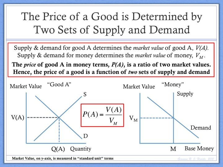
What many economists don’t seem to appreciate is that every price is a relative measurement of market value. More specifically, the price of a good in money terms is a relative measure of both the market value of the good itself and the market value of money. If the market value of the good, as measured in absolute terms, is constant and the market value of money falls, then the price of that good will rise. (See “A New Economic Theory of Price Determination” for an extended discussion of this point.)

At a macroeconomic level, the price level can be considered to be a ratio of two market values. More specifically, the price level is determined by both the market value of the basket of goods (the numerator) and the market value of money (the denominator).

In a weak economy, it is likely that there will be pressure on the numerator in our equation above: if there is less demand, then the basket of goods becomes “less valuable” in an absolute sense.

However, this does not mean that price must decline in a weak economy. Why? Prices may rise and rise significantly in a weak economy if the market value of money, the denominator in our price level equation, declines by a greater degree than the decline in the market value of goods, the numerator in our equation. (See “Will Inflation Rise or Fall in the Next Recession?” for an extended discussion of this point.)

In summary, if credit and economic growth stalls and this damages long-term economic confidence, then the value of fiat money could decline sharply, leading to a sudden acceleration in inflation.

The Value of Money and Long-Term Economic Confidence

This discussion raises a couple of obvious questions about the relationship between economic expectations and the value of money. First, what factors influence the value of fiat money? Second, why is the value of fiat money tied to long-term economic confidence?

These are topics that we have discussed in many recent posts, but we shall address them both briefly here.

The first question is discussed at length in two posts that should be read together titled “The Evolution of Money: Why Does Fiat Money Have Value?” and “What Factors Influence the Value of Fiat Money?”

In essence, the view of The Money Enigma is that fiat money is a financial instrument and derives its value from its implied contractual properties. Representative money (money backed by gold) derived its value from an explicit contract that promised a certain amount of gold on request. When we abandoned the gold standard, this explicit contract was rendered null and void.

So, why did paper money retain any value at that point? The view of The Money Enigma is that paper money retained its value because the explicit contract that governed paper money was replaced by an implied-in-fact contract.

Fiat money is a financial instrument. A financial instrument, by definition, only has value to one party because it is a liability of another. From an economic perspective, fiat money is a liability of society. More specifically, fiat money represents a proportional claim against the future output of society.

This theory allows us to begin to answer the second question raised above, namely “why is the value of fiat money tied to long-term economic confidence?

If fiat money is a proportional claim on the future output of society, then its value will be primarily determined by two variables.

The first variable is the expected rate of long-term real output growth. If fiat money is a claim to future output, then a higher expected long-term growth rate of output will make fiat money more valuable today.

The second variable is the expected long-term path of the monetary base. If every unit of the monetary base represents a proportional claim (or “share”) of future output, then expectations of higher levels of future money creation will lead to a lower value for each unit of money today.

The alternative way to state this is to say that the present value of fiat money primarily depends upon the expected long-term path of the “real output/monetary base” ratio. What determines the expected path of the “output/money” ratio? The answer is confidence in the long-term economic future of society.

If people are optimistic about society, then they should reasonably expect solid real output growth and constrained growth in the monetary base. However, if people become pessimistic about the economic future of society, then they may well expect low levels of output growth that are supported by high levels of monetary base growth. If people move from a state of long-term optimism to a state of long-term pessimism in a short period of time, then the value of fiat money will decline sharply.

In simple terms, the view of The Money Enigma is that “fiat money is only as good as the society that issues it”. What this really means is that the value of any fiat currency, and hence the price level of any fiat currency regime, is intimately tied to confidence regarding the economic future of that society. We have seen this simple principle demonstrated repeatedly. For example, think Zimbabwe in the 1990-2010 period.

While it is very unlikely that the Western World will follow a similar path to Zimbabwe, for a whole host of reasons, it does seem possible that the real test of our fiat monetary system is yet to come. If economic growth stalls as we reach the point of system-wide credit saturation, we may see the virtuous economic cycle that we have enjoyed turn into a vicious cycle of economic misery.

Why Do Prices Rise Over Time?

Since 1950, prices in the United States have risen roughly tenfold. Given this history, it would be easy for one to believe that inflation is just a natural part of economic life. But there have been many extended periods in human history where prices were either stable or even declined.

For example, prices in the United States fell at a rate of 1 per cent a year from 1879 to 1897 and then rose at a rate of little more than 2 per cent a year from 1897 to 1914 (Friedman & Schwartz, “A Monetary History of the United States”, page 91).

This begs some obvious questions. Why do prices rise over some extended periods of time and not others? More specifically, why did prices remain relatively stable while the United States adhered to a strict gold standard pre-WWI? In contrast, why did prices rise dramatically in the later half of the 20^th century as the United States abandoned the gold standard?

Milton Friedman famously remarked, “Inflation is always and everywhere a monetary phenomenon in the sense that it is and can be produced only by a more rapid increase in the quantity of money than in output.”

The long-term economic data clearly supports Friedman’s contention. But, Friedman never adequately explained why this is the case. Why should growth in the monetary base that is in excess of growth in real output lead to rising prices over extended periods of time?

The view of The Money Enigma is that the primary reason that prices rise over time is because growth in the monetary base that is greater than growth in real output acts to reduce the value of money.

The value of money acts as the denominator of the price level: as the value of money falls, prices as measured in money terms rise. If the value of money is relatively stable over time, as it generally was under a strict gold standard, then the price level is relatively stable. However, if the value of money declines significantly over time, as it has tended to do under fiat regimes, then the price will rise significantly.

Why does fiat money tend to lose value over extended periods of time? The simple answer to this question is that maintaining the value of fiat money relies on restricting the growth in the fiat monetary base and, under fiat regimes, the temptation to expand the monetary base is simply too great.

In more technical terms, fiat money is a long-duration, special-form equity instrument and represents a proportional claim on the future output of society. Measured over long periods of time, growth in the monetary base that is in excess of growth in real output will reduce the value of a proportional claim on future output, i.e. it will lead to a decline in the value of money. It is this sustained decline in the value of money that is the primary driver of inflation over long periods of time.

Every Price is a Relative Measurement of Market Value

In most of our daily life, we measure things using “standard units” of measurement. For example, we measure height in inches and weight in pounds. Inches and pounds are useful tools for measurement because they are invariable in the property that they are trying to measure. One inch is exactly the same length as it was yesterday and as it will be one year from now.

In this sense, most of the measurements that we make in our daily can be considered to be “absolute” measurements: they are made using a standard unit of measurement that is invariable in the property being measured.

However, in our economic interactions, the way we measure things is quite different.

The price of a good in money terms is a measure of the market value of that good. For example, if we know that an apple costs one dollar, then that tells us something about the value of apples.

However, while the price of a good is a measure of the market value of that good, it is not an absolute measure of the market value of that good. Why? Price is not an absolute measure of market value because our unit of measurement, “money”, is not invariable in the property that is being measured.

Unlike inches and pounds, which are both invariable in the property they are measuring, money is not invariable in the property of market value.

Therefore, the price of a good is always a relative, as opposed to an absolute, measure of market value.

What does this mean in practice?

If the price of apples in money terms is a relative measure of market value, then this means that the price of apples can rise for one of two reasons. Either (a) the market value of apples rises (each apple becomes “more valuable”), or (b) the market value of money falls (each dollar becomes “less valuable”).

The way that economics is taught today creates the temptation to ignore the second element outlined above. Traditional supply and demand theory focuses on how changes in the supply and demand for a good impact the market value of that good and, therefore, the price of that good.

What is often overlooked in this analysis is that the price of a good in money terms depends just as much on the market value of money as it does on the market value of the good itself. While it may be useful for classroom demonstrations to assume that the value of money is constant, this is not the way the world actually works.

This is particularly the case when we consider what drives prices over extended periods of time. For example, in 1950 apples in Florida cost roughly 20 cents per pound. Today, apples sell for approximately $1.50-2 per pound.

Why did apple prices increase roughly tenfold over the last sixty years? Was there “too much demand” for apples or “too little supply?” Or did something else happen? Maybe the market value of apples, as measured in absolute terms, hasn’t changed that much over that period of time. Maybe, the price of apples has risen tenfold because the value of money (the value of one US Dollar) has fallen by roughly 90% over that same period!

Arguably, the price of apples in money terms has risen tenfold over the past sixty years not because of any significant change in the value of apples per se, but because a dramatic fall in the value of our unit of measurement, i.e. a dramatic fall in the value of money.

Ratio Theory: The Price Level is a Relative Measure of Market Value

So far, we have focused only on the price of one good, the price of apples. The price of apples in money terms measures the market value of apples in terms of the market value of money. Therefore, the price of apples can rise either because (a) apples become more valuable, or (b) money becomes less valuable.

In this sense, the market value of money acts as the denominator of the price of apples. All else remaining equal, if the market value of money falls, the price of apples, as measured in money terms, will rise.

If this observation is true for the price of apples, then it is also true the price of every other good in the economy, i.e. the market value of money is the denominator of every money price in the economy.

The price of apples, the price of bananas, the price of milk… all of these prices, as expressed in money terms, are determined by both the market value of the good itself (apples/bananas/milk) and the market value of money. All else remaining equal, if the market value of money falls, then the price of all these goods, as measured in money terms, will rise.

Now, let’s think about what determines the price of a typical basket of goods, or what is often known as “the price level”.

Clearly, if the value of money is the denominator of the every money price in the economy, then the value of money is also the denominator of the price level. All else remaining equal, as the value of money falls, the price of the basket of goods will rise.

The price level is a relative measure of market value. The price level measures the market value of the basket of goods in terms of the market value of money. In this sense, we can think of the price level as a ratio of two values. The price level is determined by the ratio of the market value of the basket of goods (the numerator) divided by the market value of money (the denominator).

The key to “Ratio Theory”, as illustrated in the slide above, is isolating the market value of goods from the market value of money by measuring both in terms of a “standard unit” for the measurement of market value. Just as we measure height and weight in terms of a standard unit, so we can, at least theoretically, measure the property of market value in terms of standard unit, i.e. a unit that is invariable in the property of market value. For more on this topic please read “The Measurement of Market Value: Absolute, Relative and Real”.

In simple terms, the Ratio Theory of the Price Level implies that the price level can rise for one of two basic reasons. Either (a) the basket of good and services becomes more valuable, or (b) money becomes less valuable.

Now let’s return to original question. Why do prices rise over some periods of time and not others? More specifically, why were prices relatively stable under a gold standard and why did prices rise dramatically once the gold standard was abandoned?

The Gold Standard and Price Stability

Speaking in general terms, history indicates that prices tend to more stable, when measured over long periods of time, under a gold standard than they are under fiat monetary regimes. This is not to say that prices don’t fluctuate under a gold standard nor that there is no inflation under a gold standard, but it is true, as a general rule, that inflation has been systematically lower under true gold standard regimes than it has been under fiat money regimes.

So, why do prices tend be stable over long periods of time under a gold standard?

The view of The Money Enigma is that the main difference between a fiat money regime and a gold standard system is that, under the gold standard, the value of money is relatively constant as its value is tied to gold. Therefore, the denominator in our price level equation tends to be stable over long periods of time and the price level itself is relatively stable.

In contrast, under a fiat money system, the value of money tends to decline over time for reasons that we shall discuss shortly. As the denominator in our price level equation declines, sometimes precipitously, the price level rises.

The key principle of a gold standard is that each dollar is exchangeable for some fixed amount of gold. Under a gold standard, paper money has value because the issuing authority has made an explicit promise that paper notes are convertible into a fixed amount of gold on request.

Therefore, the value of each note is tied directly to the value of the gold. As the value of gold rises, the value of money rises. As the value of gold falls, the value of money falls.

Measured over long periods of time, the value of gold tends to be relatively stable. There are good reasons for this, as discussed in a recent post titled “What Determines the Price of Gold?”

In simple terms, gold acts a constant in sea of economic variables. More specifically, the stock of gold is relatively constant over time and, perhaps more importantly, its growth is very predictable. While the value of gold does fluctuate, gold is still the closest thing that we can find to an economic constant, especially when considered over long periods of time.

The value of gold is susceptible to sudden increases in supply, i.e. new discoveries. For example, when the New World was discovered, a large influx of gold and silver into Europe led to the “Price Revolution”. The new supply of gold and silver led to a gradual fall in the value of gold and prices, as measured in gold terms, rose roughly six-fold over a 150 year period. Nevertheless, that rate of inflation only amounted to 1-1.5% per year!

The point is that prices tend to be stable under a gold standard because the value of gold tends to be stable and, therefore, the value of money tends to be stable. If the value of money, the denominator in our price level equation, is relatively stable over time, then the price level itself is relatively stable. Economic cycles of excess demand and excess supply may lead to variations in the value of the basket of goods, the numerator in our equation, but it is the value of money, the denominator in our equation, that is the key determinant of inflation when measured over long periods of time.

Fiat Money Regimes and Inflation

If prices are relatively stable under a gold standard, then why do prices tend to rise under fiat money regimes?

Almost universally, fiat money regimes have experienced levels of inflation that are far above long-term historical averages. For example, prices in the United States pre-WWI were relatively stable, but then exploded higher in the second half of the 20^th century.

But why is this the case?

Once again, I would encourage readers to look at the price level equation below and think about what is likely to be the key difference between a gold standard system and a fiat money system.

Does seem reasonable to believe that the key difference between periods of low inflation and high inflation is the numerator in our equation? Was the value of the basket of goods relatively stable pre-WWI, but then, for some reason, broke with history and exploded higher in the second half of the 20^th century?

Or is it more plausible to believe that the difference between the two periods was the denominator in our equation, the value of money?

The view of The Money Enigma is that it is the denominator, not the numerator, which is the key driver of the price level as measured over long periods of time. More specifically, it was the collapse in the value of fiat money in the second half of the 20^th century that led to inflation well above historical averages.

Under a strict gold standard, the value of money is tied to the value of a gold and, consequently, its value tends to be relatively stable. In contrast, the value of fiat money is not pegged to the value of any real asset. Indeed, fiat money is, at least superficially, just a piece of paper.

So why does fiat money have any value and why does that value tend to decline over time?

The first part of that question is an issue that we have addressed in detail on several occasions. I would encourage people who are genuinely interested in this topic to read two recent posts, “Why Does Money Exist? Why Does Money Have Value?” and “The Evolution of Money: Why Does Fiat Money Have Value?”

In simple terms, under a gold standard, paper money represented an explicit contract that promised that it could be exchanged for gold. When the gold standard was abandoned, the explicit contract that governed paper money was rendered null and void.

So, why did paper money retain any value? It retained value because the explicit contract was replaced by an implied-in-fact contract, or “social contract”, between the holders of money and the issuer of money.

What is the nature of the implied contract that governs fiat money?

Again, this is a lengthy subject that is discussed in the “Theory of Money” section of this website. But, in simple terms, fiat money is a financial instrument: it has value as an asset to one party because it represents a liability to another party. More specifically, fiat money is a liability of society and a proportional claim on the future output of society.

This is a complicated idea, but there is a simple analogy that we can use to help us think about what determines the value of fiat money.

In many ways, fiat money is like shares of common stock. A share of common stock represents a proportional claim on the future residual cash flows of a company. In contrast, one of fiat money represents a proportional claim on the future output of society.

Over an extended period of time, if a company grows its earnings faster than it grows shares outstanding, then the value of the stock will rise. Conversely, if over a lengthy period, a company grows it shares outstanding faster than it grows its earnings, then the value of its shares will fall. Why? Each share is a claim on earnings and, ultimately, the value of each share depends on the earnings per share.

Similarly, if over an extended period of time, a society grows its real output faster than it grows its monetary base, then the value of each unit of the monetary base will rise, i.e. the value of money will rise and, all else equal, the price level will fall.

This doesn’t happen very often, especially under fiat money regimes. Rather, most of us are more familiar with the alternative scenario.

If over a long period of time, a society grows its monetary base faster than real output, then the value of money will fall. Why? The value of money falls because money, the monetary base, derives its value from an implied-in-fact contract. More specifically, money represents a proportional claim on future output. In general terms, as real output per unit of money falls, the value of money falls and, all else remaining equal, the price level rises.

In summary, the primary reason that prices tend to rise under fiat money regimes is that, over long periods of time, fiat money regimes tend to grow the monetary base at a rate that is faster than the growth in real output. Fiat money is a financial instrument and represents a proportional claim on future output. All else remaining equal, as the “real output/base money” ratio declines over time, the value of fiat money declines.

The key difference between a gold standard regime and a fiat money system is the behavior of the value of money over long periods of time.

Under a gold standard, the value of money is relatively stable because it is tied to the value of gold. In a fiat money system, the value of money is heavily influenced by political process and the “needs/wants” of our society. Inevitably, as central bankers acquiesce to the needs of the people, the monetary base grows at much faster rates than real output, leading to a decline in the value of money and a rise in the general price level.

Author: Gervaise Heddle

Is Money a Short-Duration or Long-Duration Asset?

Is the value of money more sensitive to changes in short-term expectations or long-term expectations? Is what happens in the economy today the key driver of the value of money and the price level, or are both the value of money and the price level driven primarily by confidence about the long-term economic future of society?

In last week’s post, we explored the idea that “money is only as good as the society that issues it”. More specifically, the value of any given fiat currency depends primarily upon expectations regarding the future economic prospects of the society that issues it. But is the value of money more sensitive to expectations regarding the near-term economic prospects of society or the long-term economic prospects of society?

We can state this question another way: “Is fiat money a short-duration or long-duration asset?” This may seem like a strange question to ask about money. After all, most people associate the concept of duration with fixed income securities, not “cash” (the monetary base).

However, every financial instrument, including fiat money, can be considered to possess the property of “duration”. Moreover, the duration of an asset is a critical determinant of how that asset behaves in response to changes in expectations.

The view of The Money Enigma is that fiat money is a financial instrument and a proportional claim on the future output of society. More specifically, fiat money is a long-duration instrument.

While there are a couple of ways to demonstrate that money is a long-duration asset, the simplest method is to apply what I call the “benefits-cut-off” test, i.e. imagine if it was announced that money would be no longer accepted in exchange for goods and services in one year from now or five years from now, or twenty years from now etc. and imagine what would happen to the current value of money in each of those circumstances.

Why does the duration of money matter? Well, if we understand the duration of fiat money, then we can create better models for the value of money and, consequently, the price level. More specifically, if money is long-duration asset, then we can argue that both the value of money and the price level are far more responsive to changes in confidence regarding the long-term economic future of society than they are to any change near-term economic conditions.

The Concept of Duration

The duration of an asset is the weighted average time that it will take to receive the present value of the benefits generated by that asset. The term is most commonly applied to fixed income securities. A 5-year, interest-bearing government bond is a “short-duration” asset, while a 30-year zero-coupon bond is a “long-duration” asset.

From a practical perspective, if an asset is a “short-duration asset”, then most of its value relates to benefits that will be received in the near future. Short-duration assets are highly sensitive to changes in current conditions and expectations regarding the near future, i.e. the next 2-3 years. However, short-duration assets are, as a general rule, completely insensitive to changes in long-term expectations.

In contrast, the value of a “long-duration asset” depends primarily on benefits to be received in the distant future, i.e. 10-20 years from now. The value of a long-duration asset is highly sensitive to changes in long-term expectations, but relatively insensitive to changes in expectations regarding short-term conditions.

While the concept of duration is most commonly applied to fixed income securities, it can be applied to any financial instrument. After all, the value of every financial instrument depends upon benefits that we expect to receive from that financial instrument in the future. “Duration” simply provides with a measure of the average time taken to receive the present value of those benefits.

Indeed, every financial instrument can be considered to possess the property of “duration”. For example, John Hussman often discusses the idea that equities are a very long-duration asset. In theory, the stock market should be far more sensitive to changes in expectations regarding long-term earnings growth than changes in current economic conditions and earnings.

If every financial instrument possesses the property of duration, then this raises two interesting question relating to the nature of money. Is fiat money a financial instrument? And if it is, then what is the duration of fiat money?

Fiat Money as a Financial Instrument

The view of The Money Enigma is that fiat money is a financial instrument. Every asset can be classified as either a real asset or a financial instrument. Fiat money is not a real asset and, therefore, must be a financial instrument.

The classification of assets into real assets and financial instruments is important because it relates to how an asset derives it value. Assets can only derive their value in two ways: either they derive their value from their physical properties or they derive their value from their contractual properties.

A real asset is an asset that is tangible or physical in nature. More importantly, it is an asset that derives its value from these tangible or physical properties.

In contrast, a financial instrument is, by definition, both an asset and a liability. A financial instrument derives its value as an asset from the liability that it represents to another. In this sense, the value of a financial instrument can be considered to be an artificial creation of a contract entered into by economic agents.

In simple terms, if something doesn’t derive any value from its natural or intrinsic properties, then the only way it can derive value is if it creates an obligation on a third party to deliver something of value. Indeed, this paradigm is so fundamental that it is used as the basis of classification of assets for accounting purposes.

So, where does fiat money fit in this simple paradigm? Does fiat money derive its value from its physical nature or does it derive its value from the liability that it represents to its issuer?

The view of The Money Enigma is that fiat money is a financial instrument and derives its value solely from the nature of the liability that it represents. Money is an asset to one party because it is a liability to another. More specifically, money is a liability of society and represents a proportional claim on the future output of society.

In simple terms, the cash in your pocket has value to you today because you believe that you will be able to exchange that cash for goods and services in the future. The money in your pocket represents a claim against the future output of society. This is the essence of the social contract that fiat money represents.

So, if fiat money is a financial instrument and every financial instrument possesses the property of duration, then what is the duration of fiat money?

The Duration of Fiat Money

One of the aspects of fiat money that makes it rather unique as a financial instrument is that it doesn’t entitle us to a stream of future benefits. Rather, it entitles us to a slice of future benefits. In simple terms, we can only spend the dollar in our pocket once. We can spend it today, tomorrow, one year from now or twenty years from now.

Since most of us are in the habit of spending the dollars in our pocket within a week or two, this would suggest that money is a short-duration asset. However, this simplistic form of analysis is wrong. Just because we don’t typically hold the same cash in our pockets for a long period of time, doesn’t mean that fiat money is a short-duration asset.

There are two much better ways to think about the duration of money. The first is relatively simple and involves the application of a basic test. The second is more complex and requires an appreciation of the economic concept of “intertemporal equilibrium”.

Let’s begin by discussing the first, relatively simple approach.

There is an easy test for duration of any asset. For lack of a better term, we can call this test the “benefits cut-off test”.

As discussed, a financial instrument only has value because it creates an obligation on the issuer of that instrument to deliver something of value in the future.

The benefits cut-off test involves imagining a scenario in which the issuer of that financial instrument announces that it will not to honor the liability starting x years from now and thinking about the impact that announcement would have on the current value of the security.

For example, if the government announced that, starting five years from today, it would stop paying interest and principal on all government debt, what would be the impact on the value of its debt?

Clearly, it depends on the duration of the debt. The announcement should have no impact on one-year government debt, after all, the interest and principal will be repaid well before the government stops honoring its commitments.

But what about recently issued 30-year debt? Clearly, the value of such debt would collapse. Why? Because it is a long-duration asset: most of its value is associated with payments that will be made well beyond five years from now.

Now, let’s apply the benefits cut-off test to fiat money.

As mentioned, the view of The Money Enigma is that money is a financial instrument that represents a proportional claim on the output of society. In short, fiat money is a liability of society and its value depends on society honoring its obligation to deliver output in exchange for little pieces of paper.

Now, what would happen to the value of money and, conversely, the price level, if it were announced that society would not honor money’s claim on output starting one year from now?

Think about this for a moment. What would your immediate reaction be if the government announced that cash would no longer be accepted in commercial exchange one year from now? My guess is that you would try get rid of all your cash and cash-related securities, i.e. bank deposits, as fast as possible!

The problem is that everyone else would try to do the same thing. What would happen to the value of money if everyone wants to get rid of it and no one wants to accept it? It would collapse.

If the government announced that money would no longer be accepted one year from now, then it seems reasonable to believe that there would be panic and the value of money would collapse, not in one year, but today, right now. What would happen to prices in this scenario? Prices would soar. You can imagine the scene: people offering $100,000 for a jar of peanut butter and the grocer refusing to accept it.

Let’s try a different scenario. What if it was announced that the cut off was 5 years from now? In other words, what would be the reaction if everyone learnt that money would not be recognized as a claim on output starting five years from now?

In this scenario, there might not be panic, but there probably would be an immediate drop of in the demand for money. Again, money would lose a substantial portion of its value very quickly and prices, as expressed in money terms, would skyrocket.

What about if the cut off was 10 years from now? Maybe a smaller drop in value, but still a drop in value.

Now, apply a 30-year test. Would there be a significant drop in the value of money today? Probably not. Why? Well, 30 years is a long time from now. Arguably, money could function for at least another ten years before people really start to worry about the end point.

Clearly, this exercise involves a large degree of speculation, so we won’t belabor the point. Nevertheless, it does give some credence to the view that money is a long-duration asset. The value of money is highly dependent upon the expectation of benefits, in the form of goods and services, that can be claimed with money not just months but years from now.

So, how is it possible for money to be a long-duration asset? After all, we tend to think of money as something that we can spend now or at any time we wish.

The benefits cut-off test provides a hint as to the answer: the value of money today depends upon a long chain of expected future values.

In very simple terms, I accept money from you because I think I will be able to acquire goods of value from the next person. In turn, the person who accepts that money from me does so because they think that the next person will accept it as something of value. And so a chain develops: money has value now because we believe it will have value to each successive person in the chain.

Fiat Money and Intertemporal Equilibrium

What our very basic example highlights is that the equilibrium value of money incorporates a chain of expected future values for money. More specifically, the present value of money depends largely upon the expected variable entitlement of money in distant future periods. If, as in our example, the entitlement of money drops to zero in future periods, then this has a big impact on the current equilibrium value of money.

In theory, the economy should always be in or adjusting towards a state of intertemporal equilibrium. If it is announced that society will no longer recognize money as a claim on output beginning next year, then it will lose all, or nearly all, of its value today. In essence, a state of intertemporal equilibrium is disrupted by the announcement: everyone tries to spend the money today with the result that no one can spend the money, or only at a massively reduced value.

In our simple one-year cut-off example, equilibrium is only restored once the value of money has fallen to such a degree that someone is prepared to accept it in exchange for goods or services. The price level may well have to rise by a 1000% or more in order to restore a state of intertemporal equilibrium.

Interestingly, there is another way we can leverage the concept of intertemporal equilibrium to demonstrate that fiat money is a long-duration asset. More specifically, we can use the concept of intertemporal equilibrium to demonstrate that the expected value of money in distant future periods does impact the value that we put on money today.

This process starts by investigating one of the key differences between fiat money and shares of common stock.

One of the most obvious differences between money and a traditional equity instrument is that one unit of money provides its holder with a claim to a slice, not a stream, of future economic benefits. A share of common stock provides its holder with a proportional claim to a stream of future cash flows. In contrast, one unit of money provides its holder with a one-time claim on the output of society, or a “slice” of future output.

If a financial instrument entitles its holder to a stream of future benefits, then we can create a valuation model for that asset by simply adding the present value of each of the expected future benefits in that stream.

However, if a financial instrument entitles its holder to a slice of some set of possible future benefits, then we face a different challenge: the present value of that instrument could equal one future benefit or another or another.

In essence, we are left with a question of probability: what is the probability that the holder of that financial instrument will claim any one of n different future benefits? If we know the probability of each slice being claimed (i.e. the probability of when the money will be spent), then we can calculate the present value of the asset.

So, how do we create a probability function to weight each of the possible future values of money and, thereby, determine the current equilibrium value of money? The key to the answer lies in the question itself: the concept of “equilibrium”.

Equilibrium can be thought of in one period terms, “static equilibrium”, or in multi-period terms, “intertemporal equilibrium”. It is the view of The Enigma Series that in order for the economy to be in a state of intertemporal equilibrium, the marginal holder of money must be indifferent between spending the marginal unit of money at any point in their future-spending horizon.

Think about it this way: if you would much prefer to spend the marginal dollar you receive in five years, than spend it today, then you haven’t maximized your utility and the economy is not in a state of equilibrium. In simple terms, you have an incentive to act and, by definition, the economy is not a “state of rest”.

If you have n years remaining in your life, then technically, for the economy to be a state of general equilibrium, you should be indifferent between spending money now versus spending money in any one of those future n years. Moreover, you will also be indifferent as to which of those future periods you spend the money in. For example, you will be indifferent as to whether you spend the marginal dollar in 5 years, 10 years or 20 years.

[Geeks note: Mathematically, if you are indifferent between A (spending money now) and B (spending money in 5 years) and indifferent between A (now) and C (10 years), then you are also indifferent between B (5 years) and C (10 years)].

Now, we can use this idea to create our probability distribution. If the marginal holder of money must be indifferent between spending the marginal unit of money at any point in the future n period spending horizon, then the probability that the marginal unit of money is spent in any one of the future n periods is 1/n.

At least theoretically, the probability that we spend the marginal dollar twenty years from now is the same as the probability that we spend it one year from now. Therefore, the value we put on money today will incorporate not only expectations about the value of money one year from now, but the value of money thirty or even forty years from now.

This application of equilibrium theory casts new light on the duration of money. The value of money doesn’t just depend on what we expect we might get for it one or two years from now. Rather, the value of money also depends heavily on what we might expect to get for that money many years, if not decades, from now.

In summary, the value of money depends upon long-term expectations. Fiat money is a long-duration asset and the value of fiat money is highly sensitive to changes in expectations regarding the long-term (20-30 year) economic future of society.

Fiat Money is Only as Good as the Society that Issues It

Fiat money remains one of the great enigmas of modern economics. Economists struggle to provide simple answers to basic theoretical questions such as “Why does fiat money have value?” and “What determines the value of fiat money?”

Yet, intuitively, most of us recognize that there is one simple rule-of-thumb that applies to the value or worth of any given fiat currency: a fiat currency is only as good as the society that issues it.

More specifically, the value of any given fiat currency depends primarily upon expectations regarding the long-term economic prospects of society.

If the long-term economic prospects of a society are strong, then the value of the fiat currency issued by that society is well supported. Conversely, if expectations regarding the long-term economic future of society begin to deteriorate, then the value of the fiat money issued by that society begins to fall.

We have seen this simple notion illustrated repeatedly across many different countries over many different time periods. Some examples are extreme, i.e. the total economic and societal collapse of Zimbabwe at the hands of a despotic regime and the associated destruction of the Zim Dollar. Other examples are more subtle, i.e. the recent decline of the Brazilian Real as the end of the China commodity bubble has damaged confidence in the long-term economic future of Brazil.

The question that should preoccupy economists is why is this the case? From a theoretical perspective, why is fiat money only as good as the society that issues it? And why is the value of fiat money so heavily tied to confidence in the economic future of its issuing nation?

In this week’s post, we will attempt to answer these questions by exploring the nature of the obligation that society creates when it issues fiat money. More specifically, we will discuss the nature of the social contract that fiat money represents.

The Value of Fiat Money and Long-Term Economic Confidence

While it may be hard to believe now, there was a time when Zimbabwe was a thriving and prosperous nation, at least by the standards of sub-Saharan Africa. In 1980, the year Robert Mugabe and the ZANU party took power in a landslide victory, GDP per capita in Zimbabwe was the same as that in Botswana and nearly 50% of that in South Africa. At that time, Mugabe was a hero in the minds of many Africans and represented the bright future of post-colonial Africa.

However, Mugabe’s time as Prime Minister and then President of Zimbabwe was marred by corruption and economic mismanagement. The problems became worse as Mugabe tried to hold on to power with ever more populist policies. Arguably, the most damaging of these policies was the implementation of the Fast Track Land Reform program in 2000, a program that, in effect, took the nation’s most productive agricultural land away from white owners and redistributed that land to the majority black population.

These programs of redistribution not only eroded any confidence international partners had in doing business in Zimbabwe, but also destroyed the productive heartland of the nation. Not surprisingly, confidence in the long-term economic future of Zimbabwe began to collapse.

As confidence in the long-term economic future of Zimbabwe collapsed, so did the value of the Zimbabwe Dollar, as demonstrated in the chart below.

Now, there will be many readers who might argue that it was monetary base expansion (“printing money”) that led to the collapse of the Zim Dollar. Clearly, this is important part of the story, but it is only part of the story. Why? Well, we have seen many examples recently of more developed countries (US and Japan) that have dramatically expanded their monetary base without a collapse in the value of the fiat currency of their nation.

So, what is the difference between Zimbabwe in the 2000s and the United States today? In a nutshell, the expansion of the monetary base in Zimbabwe was perceived to be “permanent” in nature. In contrast, the monetary base expansion that has occurred in the United States over the past seven years is perceived to be more “temporary” in nature, i.e. an expansion in the monetary base that will be reversed when the Fed decides that “the time is right”.

In turn, what is the key factor that determines whether markets perceive monetary base expansion to be “temporary” or “permanent” in nature? The answer is long-term economic confidence.

Today, the vast majority of market participants believe that the United States will grow and prosper over the next 20-30 years. In this context, the Fed’s expansion of the monetary base represents a blip: a policy that will be relatively easy to unwind over the years ahead. Personally, I don’t completely agree with this rosy assessment of the situation, but I think that it represents a fair characterization of what most people believe.

In contrast, in the early 2000s, confidence in the long-term economic future of Zimbabwe was collapsing. This collapse in confidence was no doubt fueled by already significant declines in GDP and money printing. But at its core, this deterioration in confidence was fueled by fundamental concerns regarding the long-term economic survival of the nation in the face of extraordinary corruption and mismanagement. In this context, every Zim dollar printed was perceived as a permanent addition to the monetary base.

In more recent times, many of us have been watching the marked decline in the value of the Brazilian Real.

Some pure monetarists might want to blame this decline in the Brazilian Real on money printing. However, while the Brazilian monetary base has quintupled over the past seven years, this expansion is almost identical to the expansion of the US monetary base over that same period!

So, once again, we need to ask ourselves if it isn’t monetary base expansion per se that drives down the value of fiat currencies, then what is the common factor? Again, my answer is that the value of a fiat currency is primarily driven by confidence in the long-term economic future of the nation that issued it.

While confidence in the long-term economic future of the United States has remained strong, confidence in the long-term economic future of Brazil has collapsed over the past 12 months. Brazil is a country that, from an economic perspective, is highly dependent upon mining and agricultural commodities. When China was booming, the outlook for Brazil was good. But as the problems in China become more acute, there are increasing doubts about the long-term economic model for Brazil.

As concerns mount regarding the long-term future of Brazil, the value of the Brazilian Real falls. Put another way, it may be that the expansion in the Brazilian monetary base over the past seven years isn’t quite as “temporary” as many originally thought it might be.

From a practical perspective, the notion the value of a currency is tied to confidence in the nation that issues it is fairly straightforward. However, from a theoretical perspective, the reason for this phenomenon is much more complex. Indeed, it is so complex that mainstream economics has struggled to explain why this relationship exists.

The mainstream view that money has value because it is accepted as a “medium of exchange” provides little basis for explaining the fluctuation in currency values. Indeed, mainstream theory struggles with the simple notion that “money has value” and the role that the value of money plays price level determination. At the other intellectual extreme, the Austrian “regression theory” of money, namely money has value because it used to have value, also offers very little scope for the role of expectations in the determination of the value of money.

Therefore, in order to explore the relationship between the value of money and long-term economic confidence, we need a different model. More specifically, we need a model of money that considers the nature of the obligation that fiat money represents and the claim that fiat money represents against the future output of society.

Why Does Fiat Money Have Value?

Let’s assume for the moment that our premise is right and that the value of fiat money is driven primarily by confidence in the long-term economic future of the society that issued it. If this premise is correct, what might this imply about the nature of fiat money?

Prima facie, it would suggest that fiat money represents an entitlement to future economic prosperity. More specifically, it suggests that fiat money represents an entitlement to the future economic output generated by society.

As discussed in the previous section, if we believe that a society will enjoy long-term economic success, then the value of the fiat currency issued by that society tends to be well support. Conversely, if serious concerns surface regarding the long-term economic prosperity of society, then its currency will begin to lose value relative to other currencies and other goods in general.

Now, if fiat money represents an entitlement to future output, then this also suggests that fiat money is an obligation. In simple terms, the holder of money can’t be entitled to an economic benefit (some portion of the future economic output of society) unless some other party is obliged to deliver that economic benefit. Who is that other party? Prima facie, it would seem reasonable to believe that it is society itself.

Think about it this way. What is the main purpose of issuing fiat money? Is it to provide a useful medium of exchange? No. Is it to help the central bank manipulate the interest rate? Maybe, but that’s a very limited view of its role. The primary purpose of monetary base expansion is as a financing tool. Society authorizes government (the central bank) on its behalf to create money in order to finance certain expenditures that are deemed to be in the interest of society. Newly printed money might be used to finance general public works, or, in current times, it might be directed towards buying government bonds.

Whatever this newly created money is used to buy, the point is that it is used as a financing tool. Prima facie, this suggests that fiat money is a “financial instrument”, an asset that has value today because it creates a future liability.

A financial instrument is both an asset and a liability. A financial instrument only has value as an asset to one party because it is a liability of another party.

The view of The Money Enigma is that fiat money is a financial instrument. Fiat money is an asset to its holder because it is a liability of society. More specifically, fiat money represents a claim against the future output of society.

In simple terms, ask yourself “Why do I go to work to earn money”? I would argue that you go to work every day because you believe that the money you earn entitles you to some portion of the future output of our society. If it didn’t, why would you bother?

In this light, it makes perfect sense that the value of the fiat money we have in our pocket should be tied to the perceived future economic prosperity of our society. If money is a claim against future output, then its value should be tied to expectations of future economic success. In other words, fiat money is only as good as the society that issues it.

We can take this analysis one step further.

As a general rule, every financial instrument represents either a fixed or variable entitlement to a future economic benefit. For example, a bond typically represents a fixed entitlement to a set of future cash flows, while an equity instrument represents a variable or proportional claim on the future cash flows of a company.

It is almost impossible to make the case that fiat money represents a fixed entitlement to the future output of society. In contrast, a plausible case can be made for the notion that fiat money represents a variable or proportional claim against the future of society.

More specifically, fiat money represents an entitlement to the future output of society and that entitlement varies according to expectations regarding the future size of the monetary base. Just as the number of shares outstanding (both now and in the future) determines the proportion of cash flow that each share will claim in the future, so the size of the monetary base (both now and in the future) determines the proportion of future output that each unit of monetary base can claim in the future.

If this theory of fiat money is correct, then we can say that the value of fiat money will be positively correlated to expectations regarding the long-term path of real output and negatively correlated to expectations regarding the long-term path of the monetary base.

In other words, the value of fiat money is a barometer for confidence in the long-term economic prospects of society.

As people become more optimistic about the long-term future of society (i.e. solid output growth and contained monetary base growth), the value of the fiat currency issued by that society should rise. Conversely, as people become more pessimistic about future economic prospects (i.e. poor economic growth and high levels of monetary base growth), the value of money should fall.

In an extreme situation, such as Zimbabwe in the 2000s, where people believe that economic activity will decline markedly and money printing will remain rampant, the value of a proportional claim on the future output of that society will collapse, i.e. the value of the currency will collapse just as the Zim Dollar collapsed in the 2000s.

Ultimately, fiat money is only as good as the society that issues it. Fiat money has value because it represents a proportional claim on the future output of society. If the market expects a society to collapse, due to rampant corruption and/or war, then the fiat money issued by that society quickly becomes all but worthless. However, if a society is doing well economically and people expect it to remain strong and prosperous for the foreseeable future, then the value of the fiat currency issued by that society should remain buoyant.

QE4: High Risk, Low Reward

The view of The Money Enigma is that the “risk/reward” of QE4 doesn’t stack up. QE4 doesn’t make sense from an economic perspective, nor does it make sense for the Fed politically.

From an economic perspective, the benefits of more QE in the current climate are likely to be very limited. The $4 trillion expansion in the Fed’s balance sheet has already had the “desired effect” of reducing the required return on risk capital down to exceptionally low level. The marginal benefit for markets and the economy of further compressing the required return on risk assets is likely to be limited.

On the cost side, an additional round of QE creates the risk of tipping long-term expectations in such a way that the value of money declines precipitously and prices rise sharply.

The view of The Money Enigma is that the inflationary response to QE1-3 was subdued primarily because the market perceived the QE experiment to be “temporary” in nature. If the market suddenly decides that QE is a more “permanent” part of the landscape, then this could have a very damaging impact on long-term economic confidence and inflation expectations.

The only circumstance in which the risk/reward of more QE may be justified is if there is a dramatic deterioration in financial market conditions (i.e. a 25%+ decline in equity markets). Nevertheless, it is not clear that, given current circumstances, the Fed could catch a falling knife even if it wanted to. Moreover, the long-term risks associated with attempting to stage-manage the market with QE4 probably outweigh any short-term benefits.

From a political perspective, the case is arguably much clearer. A decision to undertake QE4 at this point in the cycle would indicate that the Fed’s bold experiment with quantitative easing has failed. If the Fed finds itself forced into further easing before the tightening cycle has even begun, then serious questions will be asked about whether the theoretical models that justified QE1-3 were sound. Politically, this would put the Federal Reserve in a very bad position, one that the Fed will attempt to avoid at all costs.

QE4: The Problem of Diminishing Marginal Returns to Policy

The view of The Money Enigma is that the marginal economic benefit associated with another round of quantitative easing at this time is likely to be minimal. “QE4”, the term most often used for the possible next round of monetary easing by the Fed, is unlikely to have anywhere near the positive impact on markets and the economy that QE1-3 had.

In order to understand why this is the case, it is worth examining a little of the history associated with quantitative easing and thinking about the primary transmission mechanism from “more money” to “good economic times”.

The first point that we need to remember about the grand monetary experiment that is quantitative easing is that the experiment only started because the Federal Reserve had backed itself into a policy corner.

In each of the major economic cycles in the 1990s and 2000s, the Fed was very quick to cut interest rates but very slow to raise them: interest rates went down by the elevator and up by the stairs. Some people will argue that the Fed was “late” to cut interest rates on some occasions, and this may be true, but the Fed has always tended to be more aggressive when in the midst of an easing cycle than it has when in the midst of a tightening cycle.

By late 2008, this repeated pattern of placating financial markets had created an awkward situation for the Fed. In simple terms, the Fed never raised interest rates aggressively enough in the 2004-2007 period, thereby fueling the US housing bubble. As liquidity disappeared from credit markets throughout 2007 and 2008, the Fed found that it didn’t have enough traditional policy tools to deal with the situation and was forced to consider unorthodox methods of dealing with the crisis.

In November 2008, the Fed started buying $600 billion in mortgage-backed securities, an act that nearly doubled the monetary base in a very short period of time. This first round of unorthodox monetary policy, “QE1”, met with almost instant success: liquidity returned to most credit markets, equity markets rallied and the decline in economic confidence was arrested.

In this sense, QE1 was the appropriate response by the Fed, even if it was the Fed that was responsible for putting itself in this awkward position in the first place. More specifically, the risk/reward tradeoff for QE1 made sense, both economically and politically. Politically, the Fed had to do something to arrest the worst financial market conditions since the 1930s. From an economic perspective, QE1 stabilized global financial markets and helped restore order.

When the history books are written, QE1 will represent a good example of the circumstances under which monetary base expansion should be considered. “Printing money” is a dangerous tool, but it is also a powerful tool. Every now and then, complex economic systems founded upon fractional reserve banking get themselves into trouble. In times of genuine economic crisis, monetary base expansion represents an important and effective last-resort policy option.

The problem for the Fed is that it didn’t reserve quantitative easing solely for times of genuine economic crisis. Rather, in November 2010, two years after the depths of the crisis, the Fed decided to launch another round of quantitative easing, buying a further $600 billion of Treasury securities. Less than two years after this, a third round of quantitative easing commenced, but this time on a much larger scale than anything seen before, with purchases of Treasury securities rising to $85 billion per month.

By the time the Fed finished QE3, the monetary base of the United States had quintupled in seven years, a simply extraordinary and historically unprecedented rate of monetary base expansion.

So, why did the Fed become so aggressive in subsequent rounds of QE? The view of The Money Enigma is that the Fed had to up the ante because of diminishing marginal returns to monetary base expansion.

In simple terms, the primary transmission mechanism from “more money” to “good economic times” is the impact that a massive and sudden expansion of the monetary base has on the required rate of return across all risk assets. As the Fed buys government securities, the required rate of return across all risk assets falls and, all else remaining equal, the price of risk assets rise. The problem is that there is a limit to how far the Fed can depress the required return on risk assets.

For those not familiar with how financial markets operate it may seem surprising that buying government bonds will force up the price of equities. After all, what does the price of government bonds have to do with the price of stocks? The answer is “everything”.

There are two ways to think about this: we can think about it in theoretical terms or in more practical terms.

In theoretical terms, the market value of a business is determined by the net present value of future cash flows that investors expect to receive from that business. If the Fed creates money and use this money to buy government bonds, then this forces down not only the interest rate on government bonds, but forces down the risk free rate which is used as the baseline for all risk asset valuations.

We can also think about this issue from a more practical perspective.

Government bonds, corporate bonds and equities are, at least to some degree, substitutes for each other. They are not perfect substitutes, but they are substitutes. As the Federal Reserve begins to buy government bonds and forces down the interest rate on government bonds, then induces investors who invest in both government and corporate bonds to seek higher yields in corporate bonds. In turn, those investors who invest across the corporate spectrum (corporate bonds and equities) will now, at the margin, chase the higher expected return in equities, forcing up the price of equities.

In this way, the Fed’s actions create a domino effect across all asset classes: investors shift from government bonds to corporate bonds, corporate bonds to low-risk equities, low-risk equities to high-risk equities, high-risk equities to venture capital.

This whole process has a positive impact across all areas of the real economy. By lowering the required cost of capital for all investments, more investment activity is stimulated and more jobs are created.

The problem is that there are diminishing marginal returns to this approach.

QE1 worked because it stabilized the required return on risk assets. In essence, risk assets were in free fall and the Fed’s actions put a floor under prices. In late 2008, early 2009, it didn’t take much (“only” $600bn) to support the global credit and equity markets.

QE2 had a positive effect because it drove down the required return on risk assets from what many would consider to be a normal level to a low level. But the $600bn committed in QE2 didn’t really get the scale of result the Fed wanted.

Enter, QE3. In essence, QE3 represented an attempt by the Fed to drive down the required return on risk assets from a level that was already low by historical standards to a level that was exceptionally low. This third round of stimulus required a much larger commitment because, at some point, you begin to approach the limit of how far you can artificially manipulate the required return on risk capital.

So, what is the expected return to QE4?

If this view of the transmission mechanism from “more money” to “more economic activity” is correct, then the economic reward to QE4 is likely to be negligible.

The required return on risk assets is already at or near historical lows (see John Hussman’s work for a description of this). Any further expansion of the monetary base is unlikely to have a major impact on the required return on risk assets and, therefore, is unlikely to have any sustained impact on the price of risk assets.

The only scenario that may offer a higher near-term reward to further monetary base expansion would be one in which the markets fall precipitously over the next few months. In this scenario, it may be the case that QE can once again be used to “put a floor” under the market and arrest a decline in economic confidence. However, even in this scenario, it is not clear that further rounds of monetary stimulus would work.

As discussed in a recent post titled “Can the Fed Catch a Falling Knife?” the Fed can control the risk-free rate, at least under normal market circumstances. However, it is much more difficult for the Fed to control the risk premium, the premium required over and above the risk-free rate. There is a high likelihood that any attempt to manipulate the risk premium and stage-manage global equity markets will backfire, an event that could lead to a loss in market faith in the omnipotence of central banks.

QE4: Up the Ante, Raise the Risk

While the problem of diminishing marginal returns to policy is well appreciated by many in financial markets, the risks associated with additional monetary stimulus are very poorly understood.

The reason the risks of further monetary stimulus are poorly understood is because most economists and market commentators subscribe to what one might call an “expectations-adjusted Phillips Curve” or “New Keynesian” view of the world.

In essence, the New Keynesian model is one that recognises the benefits of intervention, but not the costs.

The New Keynesian view of the world is that inflation is a function of two factors: (1) aggregate demand, and (2) inflation expectations.

This view of the world implies that in a weak economy, an economy operating below full capacity, monetary stimulus is unlikely to have any impact on inflation. In this scenario, the only circumstance under which monetary policy could lead to inflation is if somehow damages “Fed credibility” (Fed credibility is the key in the determination of inflation expectations).

In other words, as long as everyone believes that the Fed will do the right thing eventually, then they can keep doing the wrong thing for as long as they like.

Ironically, there is an element of truth to this. The problem is that most economists don’t appreciate what constitutes the “tipping point”: the point at which the Fed goes from being “credible” to something “not credible”.

The view of The Money Enigma is that the tipping point is the point at which monetary base expansion goes from being something that is perceived as a “temporary” phenomenon by the markets to something that is perceived as a more “permanent” phenomenon.

QE4 could represent that magical tipping point: the point at which the market decides that QE is not some temporary experiment, but rather a permanent feature of the new world order.

Why does market perception regarding the “temporary vs permanent” nature of QE matter? It matters because expectations regarding the long-term path of the monetary base are one of the critical determinants of the value of the money that we use every day. In turn, the value of money is the “denominator” of every money price in the economy: as the value of money falls, the price level rises.

Let’s take this last point first: “the value of money matters to the determination of prices as expressed in money terms”.

While this may seem like an obvious statement, it isn’t something that you will read in standard economics textbooks. Why? Well, for a start, economics doesn’t recognize the “market value of money” as an independent variable. (See “The Value of Money: Is Economics Missing a Variable?”) At a more fundamental level, economics doesn’t recognize an explicit role for the value of money in the price determination process because most economists ignore one of the most basic tenets of economics: “price is a relative measure of market value”.

In order for a commercial exchange to occur, both parties must offer for trade something that possesses the property of “market value”. Whether it is apples for oranges, or apples for money, both items being exchanged must be perceived to possess value.

The ratio of exchange, one good for another, is determined by the relative value of the two goods. For example, if one apple is twice as valuable as one dollar, then the ratio of exchange is two dollars for one apple. This ratio of exchange is also known as the “price” of the trade. The price of apples, in dollar terms, reflects the relative market value of both apples and dollars. Importantly, the price of apples can rise either because (1) the market value of apples rises, or (2) the market value of dollars falls.

If every price is a relative measure of market value, then the price level is also a relative measure of market value. More specifically, the price level measures the market value of the basket of goods in terms of the market value of money. If we measure both the market value of the basket of goods and the market value of money in terms of a “standard unit” used for the measurement of market value, then we can express the price level as a ratio of these two values.

In essence, Ratio Theory states something that is obvious to everyone except professional economists: the value of money matters to the determination of the price level. As the value of money falls, the price level rises.

This brings us back to our key point. What determines the value of money? More specifically, what is the risk that QE4 triggers a shift in long-term expectations and could that shift lead to a sudden decline in the value of money?

The view of The Money Enigma is that fiat money is a financial instrument. In other words, it derives its value from its implied contractual properties. More specifically, fiat money is a long-duration, special-form equity instrument and represents a proportional claim on the future output of society.

What does that mean in practical terms? In simple terms, this theory of money implies that the value of the fiat money we use every day depends primarily upon two key factors.

First, the value of money is positively correlated to expectations regarding the long-term future growth of real output. If money is a claim on future output, then higher expected future output growth will make each claim (each dollar) more valuable.

Second, the value of money is negatively correlated to expectations regarding the future path of the monetary base. Importantly, the current level of the monetary base isn’t as important as expectations regarding the long-term future path of the monetary base.

This is a slightly more complicated concept, but you can think of it this way. If we expect that a company will have to issue lots of shares in the future in order to survive, then the value of those shares will decline. Similarly, if the market decides that a society will have to print lots of money (claims on future output) in order to sustain itself, then the value of the fiat money issued by that society will decline.

This comparison between money and shares is explored in several recent posts, most notably “Money as the Equity of Society”. The important point is that the value of fiat money is highly dependent upon the expected long-term path of the “output/money” ratio.

In even simpler terms, we can say that the value of fiat money is a barometer for confidence in the long-term economic prospects of society. If people become more pessimistic about the long-term (20-30 year) outlook for society, then the value of money will fall.

So, why might QE4 represent a tipping point?

The view of The Money Enigma is that QE4 could negatively impact expectations in two ways.

First, it could erode market confidence in the long-term growth of real output. After all, if the Fed just quintupled the monetary base and that wasn’t enough for the US economy to reach “lift-off”, then maybe there is a bigger problem. The initiation of QE4 might just be the factor that forces people to focus on this issue and adjust down their expectations for long-term real output growth.

More importantly, the instigation of QE4 could force a dramatic rethink on the part of market participants regarding the long-term path of the monetary base.

Up until recently, the view of the market seems to have been that QE is a temporary phenomenon, something that would be wound down in due course. But if the Fed is forced to enter into a new round of monetary expansion before any contraction in the previous expansion has even begun, then surely this will force the market to consider whether the Fed will ever be able to reduce the monetary base from its current bloated level.

The view of The Money Enigma is that the Fed must reverse the existing programs of quantitative easing, as discussed in a recent post titled “The Case for Unwinding QE”. Failure to unwind previous programs puts the US economy at risk of a significant acceleration in the rate of inflation. If the Fed follows the alternative route and decides to further expand the monetary base, then the risk of a dramatic acceleration in the rate of inflation becomes very real.

The Risk of Inflation in 2016

Is inflation or deflation the greater risk in 2016? Is it possible for inflation in the United States to accelerate in the midst of global economic weakness? And in a world of complex economic cross currents and unpredictable policy actions, how do you even begin to answer these questions?

Most market commentators overly simplify the inflation or deflation debate by making a false assumption, namely that “economic weakness = deflation” and that “economic strength = inflation”. This represents an essentially Keynesian view of the world, a view that dominates the thought process of most central bankers.

But is it really this simple? Will the inflation outcome in 2016 be determined solely by the strength of the US economy? Or is there another factor at play? A factor that is harder to observe and quantify, yet one that could have a much greater impact on the 2016 inflationary outcome than near-term economic conditions?

The view of The Money Enigma is that we can break any analysis of inflation in two parts. First, we need to consider how near-term economic conditions might impact the market value of goods. For example, if the economy deteriorates, then we need to think about how this might negatively impact the value of goods and labor. This is the traditional part of the analysis that is familiar to most commentators.

The second part of the analysis is less orthodox and requires us to consider how expectations regarding the long-term economic prospects of society might shift and how any such shift might impact the market value of money.

A shift in long-term expectations is the critical second factor that is often ignored by market commentators. Long-term economic expectations play a critical role in the determination of the market value of money. More specifically, if people lose faith in the long-term economic prospects of society, then this undermines the value of fiat money issued by that society.

In this week’s post, we will explore what might happen if this second, often silent, factor comes into play in 2016. More specifically, it will be argued that inflation could accelerate markedly in 2016 if long-term confidence is damaged.

Ironically, the global economic weakness that many believe will drive a deflationary outcome in the United States in 2016 could be precisely the factor responsible for triggering a decline in long-term economic confidence and a reacceleration in the rate of inflation.

The Risk of Inflation: A Two-Part Analysis

Any attempt to analyze the risk of inflation assumes, prima facie, that one understands the key drivers of inflation. Unfortunately, economists have been unable to reach consensus regarding the primary causes of inflation.

In very rough terms, there are three competing views regarding the primary cause of inflation. Keynesians believe that inflation is caused by “too much demand” relative to the economic potential of the economy. Monetarists believe that inflation is caused by “too much money” relative to real output. Fiscal Theorists believe that inflation, particularly severe inflation, is caused by “too much government debt” as measured relative to GDP.

Professor John Cochrane in his article “Inflation and Debt” does a much better job than I can of describing these various schools of thought and some of the problems associated with each.

While each school of thought has its own problems, the greater issue from my perspective is that each school of thought speaks a different language. More specifically, the basic price level models used by the various schools of thought don’t really talk to each other. For example, the New Keynesian expectations-augmented Philips Curve doesn’t explicitly include a role for government debt and, quite frankly, has almost completely excluded any explicit role for the size of the monetary base (in the New Keynesian world, money only matters if it impacts the interest rate).

So, in the midst of all this academic confusion, how does one begin to analyze the outlook for inflation?

The view of The Money Enigma is that we can simplify our starting point by recognizing a fundamental truth: the price level is a relative measure of market value. More specifically, the price level is a relative measure of the market value of the basket of goods in terms of the market value of money.

Mathematically, the price level can be expressed as a ratio of two values. The price level is determined by the ratio of the market value of goods V_G divided by the market value of money V_M. The key to demonstrating this is recognizing that the property of market value can be measured in absolute terms, i.e. in terms of a “standard unit” for the measurement of market value. Both the market value of goods V_G and the market value of money V_M in the equation above are measured in terms of this standard unit. You can read more about this very important concept in “The Measurement of Market Value: Absolute, Relative and Real”.

If the price level is a relative measure of two factors (the market value of goods and the market value of money), then this automatically suggests that any analysis of inflation needs to be conducted in two parts.

First, we need to consider the impact of near-term economic conditions on the market value of goods, the numerator in our price level equation. Second, we need to consider how shifts in long-term expectations might impact the market value of money, the denominator in our price level equation.

As you will see from the analysis that follows, we can use this simple two-part framework (“Ratio Theory of the Price Level”) to incorporate many of the ideas that are promoted by the various schools of economic thought. More specifically, we will explore how aspects of Keynesianism, Monetarism and Fiscal Theory can all be incorporated into a discussion of the outlook for inflation.

On that note, let’s begin our two-part analysis of the outlook for inflation in 2016.

2016 Inflation Outlook, Part One: Will Global Economic Weakness Put Pressure on the Value of Goods & Labor?

There can be no question that, over the past couple of decades, major global deflationary forces that are secular in nature have emerged and that these forces have played a key role in creating the low inflation environment that is currently being experienced in the Western World.

The opening of major European markets at the end of the Cold War, the free market revolution in China and the emergence and mass adoption of the Internet have all contributed to a more competitive world.

Moreover, none of these deflationary forces look set to reverse, at least not in the near-term. Despite political tensions between Russia and the US, it seems very unlikely that the USSR will return. In China, economic bumps all the road have been met with some unorthodox policy, but the fundamental trend towards free markets still seems to be firmly in place. As for the Internet, it is hard to imagine a world without it, despite that the fact that many of us, myself included, began our careers before email existed!

Therefore, it seems relatively safe to assume that we can extrapolate these secular trends forward for at least another decade.

The secular trends may be clear, but what about the impact of cyclical factors? Are we safe to assume that, in the near term, cyclical factors will also add to the deflationary pressures?

This is a more difficult call because it requires us to see ahead into economic conditions in 2016. Will the US economy slow further in 2016? Will China act as an anchor on global economic growth in 2016?

Frankly, many of you will be in a better position than me to answer these questions. Nevertheless, let’s assume, for the sake of argument, that economic weakness spreads further in 2016 and that the US economy slows down markedly. What would we expect the impact to be on the value of goods and labor?

Clearly, any US economic weakness in 2016 would put further downward pressure on the market value of the basket of goods, the numerator in our price level equation.

This part of the analysis is entirely consistent with the Keynesian view. If secular forces continue to drive growth in aggregate supply and these secular forces are met by a cyclical decline in aggregate demand, then we should expect an increase in slack in the economy and downward pressure to build on both the value of goods and labor.

So, is that the end of our analysis? Absolutely not.

Many market commentators (and central bankers) might stop their analysis at this point and conclude with the observation that “if the economy is weak in 2016, then the risk of deflation is greater than the risk of inflation”.

The problem with concluding our analysis at this point is that we have only considered half of the picture. Inflation is not simply a function of economic strength. If it were, then Zimbabwe would have experienced deflation as its economy imploded, not hyperinflation.

So, what is the missing link? Why is it possible for economic decline to be met with an acceleration in inflation? The answer lies in the denominator of our price level equation: the value of money.

2016 Inflation Outlook, Part Two: Will a Decline in Long-Term Economic Confidence Trigger a Sharp Decline in the Value of Money?

In order for money to be accepted in exchange, money must possess the property of market value. In a commercial exchange, you are not going to give me something of value (for example, an apple) unless I give you something of value in return. When I pay for the apple with money, you accept money because you believe that money has value, value that will be recognized the next time you try to use the money I gave you to buy something.

The value of money has a critical role to play in the determination of prices as expressed in money terms. In simple terms, if the apple I try to buy from you is worth twice as much as one dollar, then I will have to give you two dollars to pay for it. If the value of money falls relative to the value of the apple, then I will have to give you more dollars for the apple, i.e. the price of the apple in money terms rises.

We can extrapolate this simple principle to the price level. The price level is a measure of the market value of the basket of goods in terms of the market value of money. In other words, all else remaining equal, if the value of money falls, then the price level rises.

This raises an obvious question: what determines the value of money?

The answer to this question is far from obvious and is something that still eludes the science of economics. Indeed, most economists struggle to even acknowledge the “market value of money” as an independent variable, for reasons that are discussed at length in a recent post titled “The Value of Money: Is Economics Missing a Variable?”

Nevertheless, by observing the history of various fiat currencies, we can make one sweeping observation regarding the nature of fiat money: fiat money is only as good as the society that issues it.

In more specific terms, the value of fiat money depends upon confidence in the long-term economic prospects of the society that issued it.

If confidence in the future of society is strong, then the value of the currency issued by that society should be well supported. Conversely, if confidence in society’s future deteriorates, then the fiat money issued by that society will decline in value. In an extreme situation, if confidence in the economic functioning of a society collapses, the value of the fiat currency issued by that society will collapse, triggering a period of hyperinflation.

Intuitively, it makes sense that the value of the fiat money issued by our society should be intimately tied expectations regarding the economic future of our society. However, from a theoretical standpoint, explaining why this is the case is a complicated challenge.

The view of The Money Enigma is that the value of fiat money is tied to confidence in the economic future of society because fiat money represents a proportional claim on the future output of society.

Fiat money is a financial instrument: it derives its value from its implied contractual properties. Fiat money is a liability of society and a claim against the future output of society. More specifically, fiat money is a long-duration, special-form equity instrument and represents a proportional claim against the future output of society.

This theory of money, “Proportional Claim Theory”, is discussed at length in the “Theory of Money” section of this website.

From a practical perspective, the primary implication of this theory is that the value of fiat money depends upon market expectations regarding the long-term (30 year+) future path of two key variables: real output and the monetary base.

Currently, the market is optimistic regarding the long-term path of real output relative to the monetary base. Most commentators believe that the Federal Reserve will reduce the monetary base from its current extended levels over the next 10 years and that during that time real output will continue to grow at solid rates.

This combination of optimistic expectations has supported the value of the US dollar and, as a result, has helped keep a lid on prices.

The fact that the Fed has quintupled the monetary base over the past seven years has had little negative impact on the value of money because the market perceives this monetary expansion to be “temporary” in nature.

But what happens if confidence in the long-term economic future of the United States declines and the market begins to believe that the Fed’s program of quantitative easing is more “permanent” in nature? What happens if global events unravel such that the market begins to believe that the Fed won’t or can’t reduce the monetary base?

Let’s continue with the 2016 scenario that we discussed in Part One: the global economy continues to weaken, with several major countries slipping into recession, and economic growth in the United States slows to crawl speed.

This is a scenario that most economists believe will almost certainly produce a deflationary or very low inflation outcome. I agree that such a scenario would put pressure on the market value of the basket of goods. But what might happen to the value of money in such a scenario?

Arguably, a period of global economic weakness in 2016 could become a tipping point for long-term expectations regarding the structural health of the United States.

Think about these factors.

First, as we enter 2016, the Fed will have made little to no progress in reducing the monetary base. Will a global recession encourage the Fed to accelerate a reduction in the monetary base? No. In an extreme scenario, a global economic recession may encourage the Fed to further expand the monetary base.

Second, a slowdown in the rate of growth in the US will not improve the Federal budget deficit nor help to reduce the outstanding debt of the US Government. Rather, a deterioration in near-term economic conditions is likely to fuel concerns about the long-term fiscal sustainability of the United States.

Third, the Fed has spent the last five years searching for “lift off”, the magic point at which the US economic recovery becomes strong and self-sustaining. After seven years of sub-par growth, a slowdown in US economic growth in 2016 might be the straw that breaks the camel’s back: the event that causes the market to lower its long-term expected growth rate for the US economy.

What is the likely outcome of the combination of these three factors: a sharp decline in the value of money.

If the theory of money discussed above is correct and fiat money represents a proportional claim in the future output of society, then a loss of confidence in the long-term economic future of the United States could easily lead to a sharp decline in the value of the US dollar.

2016: The Balance of Probabilities

What is the outlook for inflation in 2016? Our two-part analysis suggests that there could be two conflicting trends at play.

First, it seems reasonable to expect that there will be continuing downward pressure of the market value of the basket of goods, the numerator in our price level equation. All else remaining equal, this would suggest a deflationary environment in 2016.

However, the risk is “all else remaining equal” doesn’t hold in 2016. More specifically, the risk is that global economic malaise, Fed inaction and a general loss of long-term economic confidence triggers a decline the market value of money, the denominator in our price level equation.

The ultimate outcome will depend upon which force is stronger and, perhaps more critically, the timing of how events unfold.

If the economy is weak, but long-term confidence remains strong, then the majority of market commentators may prove to be right: 2016 may be a year in which inflation remains contained. However, if weakness in the economy damages long-term economic confidence, then 2016 could be the year that inflation reaccelerates.

Author: Gervaise Heddle

Supply and Demand Theory: Is The Glass Half Empty?

The basic economic theory of supply and demand is one of those beautiful scientific ideas that can be used to explain a complex process in relatively simple terms. But does this traditional representation of microeconomic price determination overly simplify the price determination process by ignoring half of the picture? In our eagerness to simplify and explain the price determination process, have we become too comfortable with a glass that is only half full?

The view of The Money Enigma is that traditional supply and demand theory is a glass half empty. More specifically, the theory of supply and demand, as it is taught today, presents a one-sided and misleading view of the price determination process.

The good news is that supply and demand theory is a glass half full: a theory that has important things to say about the price determination process. Moreover, it is a theory that can be adapted to present a more complete view of the price determination process.

However, from a more critical perspective, the traditional representation of supply and demand, with price on the y-axis, is a glass half empty: a theory that ignores an entire market process in its rush to present a simplistic view of how a price is determined.

In a nutshell, the problem can be described as follows. Price is a relative measure of market value. By definition, this implies that every price is a relative measure of the market value of two goods. Traditional supply and demand analysis focuses on changes in the market value of only one of the goods being exchanged and assumes, at least implicitly, that the market value of the second good (the “measurement good”) is constant. At best, this represents a glass half full approach to price determination: at worst, it is a misleading glass half empty approach.

In any exchange, there are two goods: a primary good and a measurement good. The price of the primary good, in terms of the measurement good, is a relative measure of the market value of both goods.

Supply and demand for the primary good can determine the market value of the primary good, but it can not determine the market value of the measurement good. Rather, the market value of the measurement good is determined by supply and demand for the measurement good.

Consequently, if price is a relative measure of the market value of both goods, then every price must be determined by two sets of supply and demand: supply and demand for the primary and supply and demand for the measurement good (see first slide below).

Traditional supply and demand analysis implies that the price of the primary good, in terms of the measurement good, is solely determined by the supply and demand for the primary good. While this model may be useful for the purposes of classroom demonstrations, it does not represent a comprehensive model of the price determination process.

Moreover, by ignoring an entire market process (i.e., supply and demand for the measurement good) it is a model that has led to many misconceptions in economics, most notably, the idea that supply and demand for money determines the interest rate.

Overview & Introduction

In this week’s post, we will focus on the theory that every price is a function of two sets of supply and demand. This is a theory that is best understood by example. Therefore, the first section of this week’s post will be dedicated to illustrating, by way of example, how prices are determined in a simple two-good barter economy. In the second section of this post, we will apply this theory to the determination of money prices.

What Determines the Price of Apples?

Most of us are so accustomed to the idea that the price of a good is determined by supply and demand for that good that it is hard to imagine how one price could be determined by two sets of supply and demand. So, what does it mean to say that “every price is a function of two sets of supply and demand” and how do we illustrate this concept?

Let’s start by examining the key elements of the slide below.

The first idea that I want to highlight is the formula in the small red box. There are two ways to explain the formula in the red box: there is a simple version and a more technical version.

Let’s start with the simple version. In essence, the formula highlighted in the red box above states that the price of one good, in terms of another good, is simply a measure of the relative market value of the two goods.

What does this mean in layman terms?

Well, imagine that good A is apples and good B is bananas and that we live in a barter economy (an economy with no money). The formula in the red box above simply states that if one apple is twice as valuable as one banana, then the price of apples in banana terms is two bananas.

In terms of the notation above, if the market value of an apple “V(A)” is twice the market value of one banana “V(B)”, then the price of apples in banana terms “P(A_B)” is two bananas.

This shouldn’t be a controversial concept. If an apple is twice as valuable as a banana (“valuable” in the sense of market value), then I would have to offer you two bananas in order to buy one apple from you. Therefore, the price of apples in banana terms is two bananas.

If it helps, try thinking about this idea in “money terms”. If one apple is twice as valuable as one dollar, then the price of an apple is two dollars. If a year later, one apple were three times as valuable as one dollar, then the price of an apple in dollar terms would have risen to three dollars.

In more technical terms, if we can measure the market value of each good in the economy in terms of a “standard unit” for market value (a unit of measure that is invariable in the property of market value), then the price of the primary good in terms of the measurement good can be expressed as the ratio of the market value of the primary good divided by the market value of the measurement good, where the market value of each good is measured in terms of the standard unit (see slide below).

Now that we have a basic formula for “the price of apples in banana terms”, our job is to figure the mechanics by which the price of apples is determined. More specifically, what are the key market forces that determine the price of apples in banana terms?

Our simple price equation suggests that there are two different sets of market forces that we need to consider. One set of market forces determines the equilibrium market value of apples “V(A)”. Another set of market forces determines the equilibrium market value of bananas “V(B)”. The price of apples in banana terms “P(A_B)” is determined by the combination of both sets of market forces.

Clearly, one of set of market forces that would impact the price of apples is supply and demand for apples. Why is this the case? Well, let’s think about what happens if there is an increase in the demand for apples.

An increase in the demand for apples shifts the demand curve for apples to the right. All else remaining equal, the equilibrium market value of apples V(A) rises.

What happens to the price of apples in banana terms? Well, if the market value of apples rises, then apples are now more valuable relative to bananas than they were previously. Price is a relative measure of market value: therefore, the price of apples in banana terms must rise. In terms of our formula, if V(A) rises and there is no change in V(B), then P(A_B) must rise.

This scenario is easily captured by traditional supply and demand analysis. On the right hand side of the next slide, the market for apples is expressed in traditional terms with “price” on the y-axis. An increase in demand for apples shifts the demand curve to the right and the equilibrium price of apples rises.

Now, what is the difference between the market forces depicted on the left hand side of the slide above versus those depicted on the right hand? The answer is “nothing”: both diagrams are saying exactly the same thing. The only thing that is different about these two diagrams is the unit of measurement on the y-axis.

On the left hand side, market value is measured in “absolute terms”, i.e. in terms of a theoretical good (a standard unit of market value, denoted “EV”) that is invariable in the property of market value.

On the right hand side, market value is measured in “relative terms”, i.e. in terms of a good (bananas) that is variable in the property of market value.

The fundamental problem for traditional supply and demand analysis is that the traditional model must assume that the market value of the measurement good (in this case, bananas) is constant. This is, at best, a glass half full approach. Why? In the real world, the market value of the measurement good is never constant.

In order to see why the traditional representation of supply and demand is compromised, let’s think about what happens to the price of apples in banana terms when there is an increase in demand for bananas.

If there is an increase in demand for bananas, then the demand curve for bananas will shift to the right. All else remaining equal, the market value of bananas V(B) will rise. Again, this shouldn’t be controversial: if there is more demand for something and no corresponding increase in supply, then that thing becomes more valuable.

So, if the market value of bananas rises, then, all else remaining equal, what happens to the price of apples in banana terms?

The price of apples falls!

All else remaining equal, if there is more demand for bananas, then bananas become more valuable. If price is a relative measure of market value and the market value of the measurement good (bananas) rises, then, all else remaining equal, the price of the primary good (apples) in terms of the measurement good (bananas) must fall.

This simple concept is easily demonstrated in the slide above where supply and demand for both goods are plotted independently, i.e. in terms of a standard unit of market value. An increase in demand for bananas leads to a rise in the market value of bananas, V(B) rises: if the market value of apples V(A) is unchanged, then the price of apples in banana terms P(A_B) falls.

Frankly, this should be simple stuff. So, how does traditional supply and demand analysis illustrate this concept? The answer is “with difficultly”.

The traditional representation of price determination for apples implies that the price of apples is determined solely by supply and demand for apples. Therefore, according to this paradigm, what happens to the price of apples as expressed in banana terms if there is an increase in demand for bananas? The answer, it would seem, is nothing.

But, as we just discussed, this is the wrong answer. Supply and demand for bananas is a critical determinant of the price of apples if the price of apples is expressed in banana terms!

So, how can traditional accommodate changes in the market value of the measurement good?

Well, the first step is to explicitly recognize that traditional supply and demand analysis assumes that the market value of the measurement good is constant. Therefore, if the market value of the measurement good changes, then both the supply and the demand function need to be rebased to reflect the change in the market value of the measurement good.

In terms of our example, if the equilibrium market value of bananas rises, then the supply and demand curves for apples, where the supply and demand functions are both measured in banana terms, must both shift lower. Consequently, there is no change in the quantity of apples sold, but the price of apples in banana terms falls.

Once again, let’s ask the question: in the slide immediately above, what is the difference between the supply and demand functions illustrated on the left hand side and the supply and demand functions illustrated on the right hand side?

The answer is nothing: both sets of supply and demand functions are identical. The only difference between the two diagrams above is the unit of measurement, i.e. the way in which the market value of apples is measured.

While it may seem like a strange concept given the shift in the curves on the right hand side, we can say that in both cases, there has been no change in the market for apples. Supply and demand for apples, as measured in terms of an invariable unit of market value, has not changed. However, our representation of the market for apples, as depicted on the right hand side, must change. Why? Supply and demand for apples, as measured in price terms, must change because the value of the unit of measurement (the market value of bananas) has changed.

In summary, the view of The Money Enigma is that using “price” on the y-axis of supply and demand diagrams creates a misleading view of the price determination process. Rather, the y-axis unit of measurement should be a standard unit of market value, a unit that is invariable in the property of market value. In this way, supply and demand can be represented in absolute terms, an act which allows us to isolate whether changes in the price of a primary good, where that price is measured in terms of a measurement good, are due to changes in the market value of first good (the primary good) or the second good (the measurement good).

Those readers who are interested in learning more about the difference between the absolute and relative measurement of market value should read a recent post titled “The Measurement of Market Value: Absolute, Relative and Real”.

Now, let’s think about how this theory of price determination can be applied to the determination of prices our money-based economy.

The Determination of “Money Prices”

In the context of a barter economy, the key advantage of plotting supply and demand for the primary good and the measurement good separately is that it allows us to isolate whether a change in the price of a primary good, in terms of a measurement good, is due to a change in market forces for the primary good or due to a change in market forces for the measurement good.

For example, in terms of our “apples and bananas” example, plotting the market for apples and bananas in standard unit terms allows us to determine whether a rise in the price of apples is due to a rise in the market value of apples or a fall in the market value of bananas.

However, this theory isn’t just relevant to a barter economy. The notion that every price is a function of two sets of supply and demand has important implications for price determination in a money-based economy.

More specifically, it is an idea that forces us to focus on the role of the “market value of money” in the determination of “money prices” (prices as expressed in money terms) and, perhaps more importantly, how the market value of money is determined.

The idea that the “value of money” matters to the determination of prices is not something that you will see discussed at length in economics textbooks. There is a good reason for this: economics does not recognize the “value of money” as an independent variable. I won’t go into a lengthy discussion of why this is the case, but it boils down to the fact that economics doesn’t recognize how to measure the property of “market value” in absolute terms. In simple terms, if you don’t measure market value in absolute terms, then you can’t isolate the value of money as an independent variable, an issue that is discussed at length in a recent post titled “The Value of Money: Is Economics Missing a Variable?”

However, by tracing the evolution of price determination from a barter economy to a money-based economy, we can see why supply and demand for money must determine the market value of money (not the interest rate!). Furthermore, we can see that the value of money is, in effect, the denominator of every “money price” in the economy: all else remaining equal, as the value of money falls, the price of goods as expressed in money terms will rise.

Let’s go back to our original diagram: “Every Price is a Function of Two Sets of Supply and Demand”.

In a genuine barter economy, an economy with no accepted medium of exchange, this model of price determination implies that the price of apples in banana terms is a function of both supply and demand for apples and supply and demand for bananas.

Now suppose that our barter economy expands to have multiple different goods. Does this principle of price determination change? No. The price of one good, in terms of another good, depends upon supply and demand for both goods. Our pricing system may have become more complex because a matrix of prices begins to develop, but the principle regarding how each price is determined does not change.

Now imagine that one of the goods in our economy is a rock called “gold”. What determines the price of apples in gold terms? Is it (a) supply and demand for apples, (b) supply and demand for gold, or (c) both?

The answer is “(c), both”.

The price of apples, as measured in gold terms, is a relative measure of the market value of apples versus the market value of gold. Therefore, the price of apples in gold terms depends upon both supply and demand for apples and supply and demand for gold.

Does it matter that this rock called “gold” is, over a period of time, called by a different name, i.e. “money”? No. Gold must possess the property of market value in order for prices to be expressed in “gold terms”; moreover, the market value of gold must be determined by a market process, namely “supply and demand”.

The notion that supply and demand for gold/silver matters to the determination of prices in gold/silver terms is supported by historical experience. For example, during The Spanish Price Revolution, a period that began in 1470 and lasted until 1650, prices as measured in gold and silver terms rose dramatically (prices increased roughly sixfold over 150 years). This period of time coincides with a dramatic influx of gold and silver from the New World (Bolivia and Mexico).

In terms of our model of price determination, as the supply of gold and silver increased, the market value of gold and silver fell. Therefore, the price of other goods, as measured in gold/silver terms, rose: in a relative sense, other goods became “more valuable”.

Now, let’s fast forward to the introduction of “representative money”. Representative money is paper money that is explicitly backed by gold or some other real asset. Should our principle of price determination suddenly change? No.

Representative money, the first form of paper, only had value because it was a contract that promised to deliver gold. The value of this paper money moved in lockstep with gold. Therefore, we can say that the value of this paper money was determined by supply and demand. Moreover, as the value of gold fell, the value of paper money fell and prices, as expressed in money terms, rose.

At some point, the explicit promise that backed paper money was removed and “representative” money became “fiat” money. Should this shift from representative money to fiat money entirely change the principle of price determination? The simple answer is “no”.

In order for fiat money to act as a medium of exchange, store of value and medium of account, fiat money must possess the property of market value. Why fiat money has value is a complex issue that we have discussed in several recent posts including “The Evolution of Money: Why Does Fiat Money Have Value?”

Nevertheless, fiat money must possess the property of market value for us to express prices in money terms and, at the most fundamental level, it is the process of supply and demand that determines the equilibrium market value of money.

The view of The Money Enigma is that supply and demand for fiat money determines the value of fiat money. More specifically, supply and demand for the monetary base determines the market value of money, as illustrated in the diagram below.

The price of a good, in money terms, is a relative measure of the market value of that good and the market value of money. The equilibrium market value of a good is determined by supply and demand for that good. The equilibrium market value of money is determined by supply and demand for money. The price of a good, in money terms is a function of two sets of supply and demand: supply and demand for the good itself and supply and demand for money.

If you would like to read more about this theory of price determination, then please visit the Price Determination section of this website. This theory is also discussed at length in a recent post titled “A New Economic Theory of Price Determination”.

Author: Gervaise Heddle

A New Perspective on the Quantity Theory of Money

The view of The Money Enigma is that the quantity theory of money needs to be reinvented. More specifically, the traditional view of the monetary transmission mechanism is wrong and needs to be completely reexamined.

The mainstream view of the monetary transmission mechanism is, in essence, that money creation leads to excess aggregate demand that, in turn, leads to higher prices. The view of The Money Enigma is that this transmission mechanism from more money to higher prices via an increase in aggregate demand is, at best, a secondary transmission mechanism.

Rather, it will be argued that the primary monetary transmission mechanism is the impact of money creation on the market value of money. In essence, “too much money” leads directly to a fall in the value of money and a rise in the price of all goods as measured in money terms.

The “value of money” is a notion that has been lost from economic theory. Indeed, mainstream economics simply doesn’t recognize the “value of money” as an independent variable, an issue that was discussed at length in “The Value of Money: Is Economics Missing a Variable?”

In this week’s post, we will attempt to shed new light on the quantity theory of money by articulating an explicit role for the value of money in the monetary transmission mechanism.

More specifically, we will discuss the role of the value of money in price level determination and we will consider, at least briefly, a theory of money that can explain why money creation leads to a fall in the value of money on some occasions, but not on others.

While money supply and real output matter to price level determination, the view of The Money Enigma is that long-term expectations of these variables are far more important than their present level. We can only incorporate these long-term expectations into quantity theory by examining how these expectations impact the value of money and the role of the value of money in price level determination.

Hopefully, this exercise will provide readers with a new and much clearer perspective on why the quantity theory of money tends to hold over long periods of time, but not necessarily over short periods of time.

The Strengths and Weaknesses of Quantity Theory

The quantity theory of money is one of the oldest surviving economic doctrines. It is a theory that dates back to at least the mid-16^th century and it was the dominant monetary theory until the Keynesian revolution of the 1930s. A good discussion of the history of the theory can be found in a 1974 paper published by the Richmond Fed, “The Quantity Theory of Money: Its Historical Evolution and Role in Policy Debates”.

It is hard to overestimate the importance and dominance of the quantity theory of money in the history of economic thought. Yet, despite a brief resurgence of interest in the late 1960s and early 1970s, quantity theory has become the forgotten child of economics: a theory that every economist learns, but one that very few seem to regard as relevant in our modern world.

While die-hard monetarists might blame the demise of quantity theory on the rise of Keynesianism, there is a more simple truth at play: quantity theory of money, as it is traditionally presented, is flawed.

The core principle at the heart of quantity theory, the notion that there is a strong relationship between the quantity of money and the price level, is fundamental, if for no other reason than the fact that it represents one of the strongest empirical relationships to be found between major economic variables.

When measured over long periods of time, there is a clear empirical relationship between the “monetary base/real output” ratio and the price level. For this reason alone, quantity theory should always occupy a revered position in the science of economics.

However, the problems for quantity theory begin when various practitioners and market commentators attempt to apply it over short periods of time. As has been well established by recent experience, there is no strict short-term relationship between the size of the monetary base and the price level. Over the past seven years, the Fed has quintupled the size of the monetary base, yet inflation has remained subdued.

This is the point at which many commentators throw quantity theory out with the garbage. Their view seems to be that if quantity theory doesn’t work in the short run, then it is as good as useless.

This is a mistake. Quantity theory should not be abandoned just because the relationship between money and prices does not hold in the short term.

Nevertheless, the burden of proof sits with advocates of quantity theory. Supporters of quantity theory need to be able to explain why quantity theory doesn’t work in the short term. The problem is that they can’t.

Why is this the case? Well, the key issue is that current theories of the monetary transmission mechanism don’t provide supporters of quantity theory with a sound basis for defending the lack of correlation between money and prices in the short run.

The view of most monetarists today is that supply and demand for money determines the interest rate. Therefore, an increase in the supply of money must operate by lowering the interest rate. In turn, a lower interest rate must stimulate economic activity leading to an increase in aggregate demand and higher prices.

In theory this sounds great, the problem is that it doesn’t work in practice. More specifically, it doesn’t explain why an increase in the monetary base leads to an increase in prices on some occasions but not others. Moreover, this simplistic view of the monetary transmission can’t account for periods of high inflation: for example, Zimbabwe didn’t experience hyperinflation because interest rates were too low and there was “too much demand”.

The problem with monetarism as it exists today is that it begins from the wrong starting point. Far from being a true monetarist view of the world, the monetary transmission mechanism described above represents a thoroughly Keynesian view of the world.

The view of The Money Enigma is that this inherently Keynesian perspective is flawed. Supply and demand for money does not determine the interest rate. Rather, supply and demand for the monetary base determines the market value of money. In turn, the market value of money is the denominator of every money price in the economy and, consequently, the denominator of the price level.

By recognizing that the primary transmission mechanism from money to prices must involve the “value of money”, we can come up with an expectations-adjusted version of quantity theory that can explain not only why quantity theory works in the long run, but also the circumstances that are required for quantity theory to work in the short run.

Our journey towards an expectations-adjusted quantity theory of money begins at a microeconomic level. More specifically, we need to explore three ideas: (1) money possesses the property of market value, (2) every price is a relative expression of market value, and (3) the price of a good, in money terms, depends upon both the market value of the good itself and the market value of money.

Price Determination and the Value of Money

If you ask most students of economics “what determines the price of a good?” then the answer you are most likely to hear is “supply and demand for that good”. This is the way that price determination is taught across schools and colleges today. However, this basic model of price determination presents a misleading and very one-sided view of the price determination process.

The problem is that economics seems to have forgotten a simple, but easily overlooked idea, an idea that was articulated centuries ago by both Adam Smith and David Ricardo: price is a relative measure of the value of two goods.

In order for a commercial exchange of goods to occur between two people, both of the goods being exchanged must possess the property of market value. In other words, I am only going to give you something of value if you give me something of value.

In a barter economy, I might have apples and you might have bananas. The ratio of exchange, apples for bananas, will depend upon the relative market value of apples and bananas at that time. For example, if an apple is twice as valuable as a banana, then the ratio of exchange is two bananas for one apples and the “price of apples in banana terms” is “two bananas”.

The price of apples in banana terms can rise for one of two basic reasons: either (a) the value of apples rises, or (b) the value of bananas falls.

Think about this for a moment. If bananas become less valuable in our community (there is a huge crop this year), then, all else remaining equal, you will have to offer me more bananas for each apple. Therefore, the price of apples in banana terms will rise.

In a money-based economy, the principle is no different.

In order for people to accept money in exchange for goods, money must possess the property of market value. For example, I wouldn’t accept money from you in exchange for my apples, unless I believe that money itself has value.

The ratio of exchange, apples for money, depends upon the relative market value of apples and money. If an apple is twice as valuable as one dollar, then the price of apples in dollar terms is two dollars. Moreover, the price of apples in dollar terms can rise because either (a) the market value of apples rises, or (b) the market value of money falls.

Mathematically, the price of a good in money terms is a ratio of two values (see following slide). The numerator is the market value of the good itself. The denominator is the market value of money.

The key to illustrating price determination in this way is recognizing that the property of market value can be measured in both relative and absolute terms. On the right hand side of the equation above, the market value of the good and the market value of money are both isolated as independent variables by measuring the market value of each in absolute terms. This is a rather complicated idea and I would strongly recommend that you read one of my earlier posts titled “The Measurement of Market Value: Absolute, Relative and Real” in order to more fully appreciate this concept.

This basic notion (price is a relative measurement of the market value of two goods) suggests that there are, in fact, two market processes at play in the determination of any price.

For example, in the case of the price of apples in money terms, one market process is determining the market value of apples, while another, completely different process, is determining the market value of money. The price of apples, in money terms, depends upon the equilibrium point that is found in both of these distinct processes.

Put another way, we can say that every price is a function of two sets of supply and demand. The price of one good (the primary good) in terms of another good (the measurement good) is a function of both supply and demand for the primary good and supply and demand for the measurement good.

The slide above presents the general version of this theory of price determination. Supply and demand for good A, the primary good, determines the equilibrium market value of good A. Supply and demand for good B, the measurement good, determines the equilibrium market value of good B. The price of A in B terms is determined by the ratio of these two market values. Therefore, the price of A in B terms is determined by two sets of supply and demand.

In the case of a money-based economy, the measurement good most commonly used is money. Money must possess the property of market value in order for it to be used as a medium of exchange. The view of The Money Enigma is that the market value of money is determined by supply and demand for the monetary base.

If you are interested in learning more about this microeconomic theory of price determination then I would encourage you to visit the Price Determination section of this website.

For now, the key point that matters is that the price of a good in money terms depends upon both the market value of the good itself and the market value of money. The price of a good in money terms can rise because either (1) the good itself becomes more valuable, or (2) money becomes less valuable.

If this microeconomic theory of price determination is correct, then we can extend it to the determination of the price level. After all, the price level is merely a hypothetical measure of the overall price of the basket of goods.

If every price is a relative measure of market value, then the price level is also a relative measure of market value. More specifically, the price level is a relative measure of the market value of the basket of goods in terms of the market value of money.

Rethinking the Monetary Transmission Mechanism

In simple terms, the slide above implies that the price level can rise for one of two reasons: either (1) the market value of the basket of goods rises, or (2) the market value of money falls.

While this model of price level determination may seem simplistic, it does open up an important question regarding the way in which monetary policy operates. More specifically, does an expansion of the monetary base lead to a rise in prices because (a) lower interest rates drive higher aggregate demand which leads to a rise in the market value of goods, or (b) does an increase in the monetary base somehow lead to a fall in the market value of money?

In more technical terms, does an increase in the monetary base impact the numerator (“V_G”) or the denominator (“V_M”) in our price level equation? Does it impact both? And if it does impact both, then which represents the primary monetary transmission mechanism from “more money” to “higher prices”?

We will consider the reaction of the market value of money (the denominator) to an increase in the monetary base in a moment: it is a complicated subject and we need to spend quite a bit of time thinking about it. But before we do, let’s think about how the market value of the basket of goods (the numerator) might respond to an expansion of the monetary base.

In order to assist us in this process, we are going to introduce the “Goods-Money Framework” (see slide below). In essence, the Goods-Money Framework represents an adaptation of traditional aggregate supply and demand analysis. On the left-hand side of the slide below, aggregate supply and demand determine the equilibrium market value of the basket of goods. On the right-hand side, supply and demand for money determine the market value of money. As discussed, the price is determined by the ratio of these two values.

Let’s focus on the left hand side of the slide above and think about how the equilibrium market value of goods (“V_G”) is likely to respond to an expansion in the monetary base.

The traditional Keynesian view would suggest that an expansion of the monetary base leads to a fall in interest rates. In turn, a fall in interest rates leads to an increase in aggregate demand. In terms of our slide above, the aggregate demand curve shifts to the right and the market value of the basket of goods rises. Implicitly, the Keynesian view assumes that the market value of money is constant (I say “implicitly” because Keynesian theory doesn’t recognise a role for the “value of money” in price determination). Therefore, any rise in the market value of goods is reflected as a rise in the price level.

As far as the traditional Keynesian view is concerned, this is where the story ends. An increase in money supply leads to higher demand and higher prices. The problem is that this story completely ignores the impact of lower interest rates on the aggregate supply curve.

In the real world, lower long-term interest rates not only lead to an increase in aggregate demand, but also lead to an increase in aggregate supply. In terms of our slide above, a fall in interest rates moves both aggregate demand and aggregate supply curves to the right and the impact on the equilibrium market value of goods is uncertain.

Lowering the long-term interest rate on government securities does more than just reduce mortgage rates and stimulate consumer spending: it also reduces the required return on capital for all businesses. Lowering the required return on capital stimulates expansion by existing businesses and lowers the bar to the start up of new businesses. What is the end result of all this new business activity? More supply!

When the central bank lowers the long-term interest rate by creating money and buying government securities, it effectively lowers the long-term risk free rate, a core component of the long-term required rate of return on risk assets, thereby encouraging business formation and driving an increase in aggregate supply.

Therefore, if Keynesian economists were sincere about the impact of lower interest rates, they would recognize that lower interest rates lead to both an increase in aggregate demand and aggregate supply and that the impact of monetary expansion on the absolute market value of the basket of goods is uncertain.

If this is the case, the traditional monetary transmission mechanism that is postulated by mainstream macroeconomists (more money, lower interest rates, more demand) is at best a secondary mechanism, and at worst is completely irrelevant.

Clearly, this analysis has an important implication.

If the numerator in our price level equation (the market value of the basket of goods) doesn’t act as the primary transmission mechanism from more money to higher prices, then it must be the market value of money, the denominator in our price level equation, which acts as the primary monetary transmission mechanism.

But how does “more money” impact the value of money? And if monetary base expansion should lead to a fall in the market value of money, then why have we not experienced this over the past seven years?

What Determines the Value of Money?

Those of you who are familiar with The Money Enigma will know that this is a topic that has been discussed at length over the past six months. If you want to take the crash course on this topic, then I would suggest reading “The Evolution of Money: Why Does Fiat Money Have Value?” and a follow-on post titled “What Factors Influence the Value of Fiat Money?”

For the purposes of this exercise, we will briefly discuss the nature of fiat money and how the value of fiat money is determined and then we will discuss the implications of this theory for quantity theory and the monetary transmission mechanism

The view of The Money Enigma is that fiat money is a financial instrument and derives its value solely from the nature of the liability that it represents. Fiat money is an asset to one party because it is a liability to another: fiat money is, from an economic perspective, a liability of society and represents a claim on the future output of society. More specifically, fiat money is a long-duration, special-form equity instrument and a proportional claim on the future output of society.

Every asset is either a real asset or a financial instrument. Real assets derive their value from their physical properties; financial instruments derive their value from their contractual properties.

The view of The Money Enigma is that this paradigm governs the way in which every asset, including money, derives its value. In ancient times, money was a real asset: money was a commodity (such as rice or silver) that derived its value from its physical properties.

The problem with this “commodity money” is that it restricted the ability of governments to spend (you can’t spend gold you don’t have). However, at some point, governments found a way to get around this problem: issue paper notes that promise to deliver gold on request. By issuing this first form of paper money, known as “representative money”, governments could aggressively expand their spending.

This first paper money was a financial instrument. It derived its value from its contractual properties. More specifically, it represented an explicit promise to deliver a real asset on request.

Ultimately, the issuance of representative money also limited the amount of money that governments could create. Therefore, at some point the gold convertibility feature was removed. This point marks the shift from representative money to fiat money.

In effect, the explicit contract that governed representative money was rendered null and void. So why did paper money maintain any value? The view of The Money Enigma is that the explicit contract that governed representative money was replaced by an implied-in-fact contract that governs fiat money to this day.

Fiat money is not a real asset and does not derive its value from its physical properties. Therefore, prima facie, fiat money is a financial instrument and must derive its value from its contractual properties, even if that contract is implied rather than explicit.

The exact nature of the implied-in-fact contract that governs fiat money is difficult to unravel. It is an issue that is discussed at length in the “Theory of Money” section of this website. However, in simple terms, the view of The Money Enigma is that fiat money is a liability of society and represents a claim against the future output of society.

More importantly, fiat money represents a variable entitlement to future output. In this sense, fiat money can be considered to be similar to shares of common stock: fiat money is a proportional claim on the future output of society, just as a share of common stock is a proportional claim on the future cash flow of a company

While there are important differences between the two, this concept can help us think about the factors that influence the market value of money, the denominator in our price level equation.

For example, if this theory is correct, then the value of fiat money is determined primarily by expectations regarding the long-term future path of two economic variables: real output and the monetary base.

In simple terms, future real output is the cake and the size of the future monetary base represents the number of slices the cake must be cut up into. If people become more optimistic about the long-term rate of economic growth, then the market value of money rises. Conversely, if people believe that long-term monetary base growth will be higher than previously anticipated, then the market value of money will fall.

The other important implication of this theory is that expectations regarding the long-term path of money and real output are far more important than current levels of money and real output in the determination of the value of money. Money is a long-duration asset and, like all long-duration assets, its value primarily depends on long-term expectations, not current conditions.

Why does this matter to quantity theory? Well, it may just be the missing piece that explains why quantity theory works well over long periods of time, but not short periods of time.

An Expectations-Adjusted Quantity Theory of Money

Let’s start by thinking about why the quantity theory of money works over long periods of time.

If the theory of money articulated above is correct, then for any long period of time (30 years+), an increase in the monetary base that is far in excess of the increase in real output should lead to a significant fall in the market value of money and, correspondingly, a significant rise in the price level.

If money is a proportional claim on economic output and, over a long period of time, the growth in the number of claims (the monetary base) far exceeds the growth in the economic benefit (real output), then one would reasonably expect the value of each claim to fall considerably as measured from point to point over that extended period of time.

Moreover, since the price level is a relative measure of the market value of goods in terms of the market value of money, one would also reasonably expect the price level to rise considerably over that same time period, assuming there was no reason for a massive collapse in the market value of goods.

In summary, quantity theory works in the long term because the market value of money roughly tracks the ratio of “real output/base money” over the long term.

However, the quantity theory of money breaks down over short periods of time. The reason for this is that short-term variations in the value of money are primarily driven by shifts in long-term expectations.

If you take a long hard look at the equation of exchange (the core equation of quantity theory), the one thing that should strike you about it is that it allows no explicit role for expectations in the determination of the price level.

If interpreted literally, then the equation of exchange implies that the price level is a function of only three variables: the current level of real output, the current level of money supply, and the current level of the velocity of money.

However, nearly all economists would agree that expectations play a key role in price level determination. Intuitively, it simply does not make sense to believe that prices across our economy have nothing to do with the expectations of economic agents.

So, how do we incorporate a role for expectations in the quantity theory of money?

The answer is to go back to our simple model of price level determination and think about how an increase in the quantity of money (an expansion of the monetary base) might impact both the numerator and the denominator in our price level equation.

As discussed earlier, if the numerator in our equation is relatively unresponsive to monetary policy, then it must the denominator in our equation, the market value of money that acts as the transfer agent from “more money” to “higher prices”. But we also know that “more money” (an expansion in the monetary base) does not automatically lead to a sudden fall in the value of money.

So, what are the circumstances in which an expansion of the monetary base will lead to a decline in the market value of money?

In simple terms, the rule of thumb is that an increase in the monetary base will only lead to a decline in the market value of money if that increase is believed to be “permanent” in nature. Conversely, an expansion of the monetary base will have little to no impact on the market value of money is that increase is believed to be “temporary” in nature.

Money is a long-duration asset. The value of money depends primarily not upon what is happening today, or is expected to happen in the next couple of years, but what is expected to happen over the next 20-30 years. More specifically, money is a long-duration, variable entitlement to future output. The value of money depends primarily upon expectations of the long-term path of both real output and the monetary base,.

In and of itself, a change in the current level of the monetary base is largely irrelevant to current market value of money. What really matters is how that change in the monetary base impacts expectations regarding the long-term path of the monetary base.

Putting this in the context of quantity theory, the conclusion we can draw is that it is not an increase in money supply per se that leads to an increase in the price level (although this will tend to be true when measured over long periods of time). Rather, the price level will rise if a monetary policy shift is deemed by the markets to indicate that the future growth of the monetary base will be higher than previously anticipated. Such a shift in expectations will lead to an immediate decline in the market value of money and, correspondingly, a sudden rise in the price level.

In summary, quantity theory is an important idea, but it needs to be modified to reflect the fact that expectations matter. More specifically, long-term expectations regarding the future economic prospects of society are the key determinant of the market value of money, the denominator of the price level. Moreover, it is the market value of money that acts as the primary transmission point from “too much money” to “higher prices”, whereas the interaction between monetary expansion and aggregate demand is, at best, a secondary transmission mechanism.

Author: Gervaise Heddle

Can the Fed Catch a Falling Knife?

In a post written three months ago “Has the Fed Created the Conditions for a Market Crash?” we discussed how the Federal Reserve’s program of quantitative easing had set up the perfect conditions for a stock market crash.

Given the recent turmoil in markets, it seems like a good time to think about how the Fed might react if major declines continue across global share markets. What will the Fed do if equity markets decline by 20% or 30% over the next few weeks or months? Moreover, how effective will any actions taken by the Fed be in circumventing these declines?

Historically, major stock market crashes (1929, 1987, 2001) have been preceded by a tightening of monetary conditions. What makes this time different is that the weakness in equity markets has not been preceded by any tightening of monetary policy: interest rates have not been raised and the monetary base has not been reduced.

Indeed, Fed policy over the past six years has been explicitly designed to lower required returns on risk capital, thereby boosting asset prices and, hopefully, real economic activity.

However, if the required rate of return on risk capital rises sharply at a point where Fed policy is still highly accommodative, then does this begin to make Fed policy look impotent? Will the markets lose faith in the Fed’s ability to manipulate desired market outcomes?

In the short term, the Fed should retain effective control over the risk free rate. However, it may be very difficult for the Fed to manage the “risk premium”, or the return that is required over and above the risk-free rate by investors in risk assets.

In the long term, the Fed faces an even greater challenge. The Fed’s likely reaction to a market collapse is either “do nothing” or “do more QE”. However, if the markets begin to believe that the Fed tightening cycle is pushed out “indefinitely”, then this could trigger a sharp acceleration in the rate of inflation. In this worse case scenario, the Fed could lose control over both the risk premium and the risk-free rate.

The view of The Money Enigma is that the markets perceive the current bloated level of the monetary base to be “temporary” and that it is this perception that is primarily responsible for holding inflation in check over the past six years.

A stock market crash is just the type of even that could change the perception that the Fed’s program of monetary base expansion is “temporary” in nature. If the markets suddenly decide the current level of the monetary base represents the “new normal”, then this shift in expectations could drive a decline in the market value of money and a sharp rise in the rate of inflation.

Dear Fed, What Happens Now?

Market events over the past few days have highlighted an interesting dilemma for the Fed. What does the Fed do when a policy explicitly designed to boost the price of risk assets suddenly stops working?

Over the past six years, the Federal Reserve has pursed an ambitious and largely experimental monetary policy called quantitative easing. Quantitative easing is designed to stimulate economic activity by suppressing the required return on risk assets, thereby encouraging new investment and business formation. Indeed, boosting asset prices by artificially forcing down the long-term risk free rate on capital is the “primary transmission mechanism” of quantitative easing.

As discussed in a recent post titled “Has the Fed Created the Conditions for a Market Crash?” the purchase of long-term fixed interest securities by the Fed forces down the required return on capital across all asset classes, thereby boosting the price of risk assets. In effect, quantitative easing creates a waterfall effect as investors are forced out of bonds and into more risky investments such as equities and private equity.

Quantitative easing only “works” from a policy-makers perspective if it boosts asset prices and confidence in the long-term economic outlook.

But, what happens if the markets crash and economic confidence is eroded before the Federal Reserve begins the process of reversing quantitative easing?

In this week’s post, we will think about both the short-term and long-term consequences associated with a significant market correction and the Fed’s likely response to this failure of quantitative easing.

Fed Tactics and Short-Term Outcomes

Can the Fed catch a falling knife? If global equity markets continue to fall over the next few weeks, what can the Fed do to arrest the panic?

In the very short-term, there are several tactics that the Fed could employ in an attempt to calm the markets.

First, the Fed could begin by hinting that any interest rate rise in September would be premature. However, this is already largely priced into markets at the time of writing. Therefore, in order to have any meaningful impact, the Fed will probably need to talk down the near-term prospects for the global economy and express concerns about the recent level of global market volatility. The markets will, probably correctly, read this as code for “no interest rate rise this year”. If this doesn’t work, then the Fed could officially rule out an interest rate rise for the next 6-12 months.

If the declines in the equity markets continue, then the Fed could adopt more aggressive tactics. The Fed could begin to suggest that further rounds of quantitative easing are back on the table. It is likely that this would have some short-term positive impact on markets because so many people got caught on the wrong side of the QE trade the first time.

In an extreme scenario, one where markets are down 25-30% from their peak in a short period of time, the Fed could announce a surprise round of quantitative easing designed to “stabilize global financial markets”.

It seems likely that the Fed will employ some combination of these tactics if market declines continue. However, the problem is that none of these short-term tactics really address the key issue.

While the Fed can control the risk-free rate (at least in the current environment) it is almost impossible for the Fed to control the risk premium that is required over and above the risk-free rate.

Over the past few years, the required risk premium has been compressed as investors have chased yield and become more and more complacent about the ability of the Fed to control market outcomes. However, when the risk premium rises sharply in a short period of time, it is very difficult for policy makers to restore it to its previous level in a timely manner.

If the Fed really wants to stop a dramatic decline in the global equity markets, it must make some attempt at manipulating the required risk premium. But given the current design of quantitative easing, this is almost impossible.

The Fed could attempt to control the required risk premium by using additional rounds of monetary base expansion to buy risk assets. In simple terms, the Fed could print money and use it to buy stocks. But this takes the Fed down an even more experimental and dangerous path.

Alternatively, the Fed could simply engage in further rounds of traditional quantitative easing: expanding the monetary base and using the proceeds to buy long-term government securities.

In the near-term, such a response would, at the margin, have some positive impact on risk assets as the purchase of government securities further compresses the risk-free rate, a core component of the required rate of return for any asset.

However, the marginal benefit from such action may be minimal. The risk-free rate is already near historical lows. Moreover, there is no guarantee that lowering the risk-free rate would also lead to any compression in the required risk premium.

In summary, there are several tactics the Fed could adopt to stabilize markets in the short-term. However, none of these tactics are likely to be able to “fix” the core problem, namely, preventing the normalization of the required risk premium.

Moreover, if the Fed does attempt to “catch the falling knife”, then there is a good chance that the Fed will end up with blood on its hands.

In the next section we will consider the possible long-term consequences should the Fed choose to chase the equity market down the rabbit hole. More specifically, we will examine why the long-term marginal cost of more quantitative easing will almost certainly outweigh any short-term marginal benefit.

Fed Strategy and Long-Term Consequences

Over the past six years, the Federal Reserve has quintupled the US monetary base. This represents an extraordinary acceleration in the rate of growth of the monetary base compared to the historical average of roughly 6% per year. So, why hasn’t this dramatic expansion in base money triggered a sharp rise in the rate of inflation?

The view of The Money Enigma is that the only reason the Fed has been able to get away with this aggressive policy and avoid a sharp acceleration in the rate of inflation is because the market believes that the extraordinary recent expansion in the monetary base is “only temporary”.

Moreover, if an event occurs that changes this perception, i.e. if people begin to believe that the recent expansion in the monetary base is more “permanent” in nature, then the value of money will decline sharply and inflation will accelerate dramatically.

A stock market crash is precisely the type of event that could trigger such a shift in expectations.

A few weeks ago, the consensus view was the Federal Reserve would begin tightening monetary policy “any day now”. Most market commentators were calling for the first interest rate rise in nine years to occur next month. This would mark the beginning of a tightening cycle that, ultimately, would see the Fed significantly reduce the size of the monetary base.

Fast-forward to today and perceptions are already shifting. Not only are markets beginning to contemplate no rate rise this year, but respected economic commentators such as Larry Summers are saying, and I quote, “it is far from clear that the next Fed move will be a tightening” (source: twitter).

While it is a matter of speculation, it is not hard to believe that should the equity markets decline a further 10-20% over the next few weeks, there will be enormous pressure on the Fed to stabilize markets by embarking on a new round of quantitative easing. Moreover, if this outcome does eventuate, then it is not hard to believe that market participants will begin to doubt that the Fed will ever restore the monetary base to its previous pre-QE growth path.

While this may sound like a subtle and rather innocuous shift in expectations, the view of The Money Enigma is that this simple shift in expectations regarding the long-term path of the monetary base could mark the starting point a whole new era in global economic affairs. More specifically, it could mark the end of the “low inflation” era and the beginning of a new “high inflation” era.

So, why do expectations regarding the long-term growth path of the monetary base matter to inflation?

In order to understand this point, we need to cover a lot of theory. Given time constraints, we will only touch on the key points today, but those that are interested might want to read two earlier posts, namely “Does Too Much Money Cause Inflation?” and “Why is there a Lag Between Money Printing and Inflation?”

The first concept that must be appreciated is that price level is highly dependent upon the “value of money”. More specifically, the price is a relative measure of the market value of the basket of goods in terms of the market value of money. In mathematical terms, the price level is a ratio of two variables: the market value of goods (numerator) and the market value of money (denominator).

In simple terms, all else remaining equal, the price level rises as the value of money falls and the price level falls as the value of money rises.

For those who are new to The Money Enigma and are not familiar with the “market value of money” expressed as an independent variable, I suggest that you read last week’s post titled “The Value of Money: Is Economics Missing a Variable?”

The second theoretical issue that must be addressed is the nature of fiat money itself. More specifically, why does fiat money have value and what factors influence that value? In other words, what determines the value of the denominator in our price level equation above?

These are questions that we have discussed at length in many recent posts. Readers can find an in-depth discussion of these issues in the “Theory of Money” section of this website, so let’s just focus on the high level points.

The view of The Money Enigma is that fiat money is a financial instrument and derives its value from an implied-in-fact contract. More specifically, fiat money is an economic liability of society and represents a proportional claim on the future output of society.

In simple terms, the value of the money in your pocket depends on long-term confidence in the future economic prospects of society. If money represents a “proportional claim on future output”, then its value is intimately tied to perceptions regarding the long-term economic prosperity of society.

One of the key implications of this theory of money is that the value of money is critically dependent upon expectations regarding the long-term future path of real output relative to the long-term future path of the monetary base.

Until a few weeks ago, the consensus view was that over the next 20-30 years real output growth would be solid while growth in the monetary base, as measured from current extended levels, would be very low. Indeed, most people would have expected that over the next 10 years, real output would grow while the monetary base would decline. These expectations have played a key role in supporting the value of money and keeping a lid on inflation.

The risk today is that a stock market crash could push both of these expectations in the wrong direction.

A major correction in global equity markets may prompt investors to revisit assumptions regarding the long-term growth of the major Western economies. Moreover, a sharp correction in markets could trigger a massive revision in the way that investors think about the future path of the US monetary base.

If investors decide that the Fed will continue to grow the monetary base over the next ten years, rather than reduce the monetary base, then this could trigger a sudden and violent decline in the market value of money.

As discussed earlier, the market value of money is the denominator in our price level equation. A sharp decline in the market value of money could easily overwhelm any deflationary trends in the goods market, leading to a sudden pick up in the rate of inflation.

In summary, investors who believe that the Fed will come to the rescue and catch the falling knife may be in for a nasty surprise. A new program of monetary base expansion may not only prove to be ineffectual in putting a floor under the market, but could also become counterproductive as it acts as a tipping point for expectations regarding long-term monetary base growth, thereby pushing the economy into a new high-inflation era and badly damaging the credibility of the Federal Reserve.

The Value of Money: Is Economics Missing a Variable?

If money has value and if the value of money is an important factor in the determination of prices in money terms, then why doesn’t economics officially recognise the value of money as a variable in its equations? Moreover, why doesn’t economics clearly explain the role of the “value of money” in the determination of money prices and foreign exchange rates?

If you look for the term “value of money” in an economics textbook, you won’t find very much. Indeed, the standard economics textbook has little to say about the “value of money” and its role in price determination.

The reason for this is simple: economics simply doesn’t recognise “the value of money” as an independent variable.

You might ask, “How is that possible? How can economics overlook a concept that seems so fundamental?” The answer to this question is rather complicated, but it boils down to the following.

In order to isolate the “value of money” as an independent variable, economics needs to measure the property of market value in absolute terms. In order to measure market value in absolute terms, economics must adopt a “standard unit” for the measurement of market value, something which economics has not done.

Almost universally, economics measures the property of “market value” in relative terms. For example, the price of a good, in money terms, is a relative measure of the market value of that good in terms of the market value of money. Similarly, the price level is a relative measure of the market value of the basket of goods in terms of the market value of money.

In both cases, economics is measuring the market value of a good or goods in terms of the market value of money, i.e. both measurements are relative in nature.

So, how does economics measure the market value of money? The most common way to do this is something called the “purchasing power of money”. The problem is that the “purchasing power of money” is also a relative measure of market value. More specifically, the purchasing power of money measures the market value of money in terms of the market value of the basket of goods. (The purchasing power of money is simply the reciprocal of the price level, itself a relative measure of value).

The problem with measuring the value of money in relative terms is that it does not allow us to isolate the “value of money” as an independent variable.

For example, the purchasing power of money can fall because either (a) the market value of money falls, or (b) the market value of the basket of goods rises. The purchasing power of money does not isolate the value of money as an independent variable: rather, it muddies the waters by mixing the value of money with the value of goods.

The view of The Money Enigma is that economics can only isolate the value of money as an independent variable by measuring the market value of money in absolute terms, that is to say, in terms of a “standard unit” for the measure of market value.

Why does this matter? Well, isolating the “value of money” as an independent variable opens a number of doors. First, it encourages us to think about why money has value and what determines that value. Second, it forces us to think about an explicit role for the value of money in the determination of prices and foreign exchange rates. Finally, and most importantly, it allows us to shed new light on existing economic theories such as the quantity theory of money.

How Do We Measure the “Value of Money”?

In our everyday life, most of us are accustomed to measuring the value of goods and services in money terms. An apple is worth one dollar. A taxi ride across town costs twenty dollars. Indeed, money is so universally accepted as a medium of exchange and unit of account that we almost instinctively measure and compare the value of economic goods in money terms.

Therefore, when somebody asks us, “how do you measure the value of money?” most of us need to pause and think for a moment. After all, how do you measure the value of something that is itself used as the measure of value?

The most common answer to this question goes something like this: if we can measure the value of goods in money terms, then we can measure the value of money in goods terms.

The value of money, in terms of the basket of goods, is known as the “purchasing power of money” and it is a popular method for measuring the value of money.

Another way to measure the value of a currency is to measure it in terms of a different currency. A foreign exchange rate is, in essence, a way of measuring the value of one type of money in terms of another type of money.

The purchasing power of money and foreign exchange rates both represent valid ways of measuring the “value of money”. However, there is a problem with this approach. Both of these measures are relative measures of value.

The purchasing power of money measures the market value of money in terms of the market value of the basket goods. A foreign exchange rate measures the market value of money in terms of the market value of another currency. In both cases, we are measuring the value of money in relative terms and, therefore, both measures are dependent upon not only the value of money, but also the value of the measurement good (the basket of goods or the other currency).

In other words, we have not isolated the “value of money” as an independent or standalone variable. Why this matters is something that we will discuss later, but first let’s consider how we might isolate the value of money as a standalone variable.

The Measurement of Market Value: Absolute versus Relative

If a physical property can be measured in relative terms, then it can also be measured in absolute terms. If we can measure the market value of money in relative terms, then we should also be able to measure the market value of money in absolute terms. Moreover, by measuring the market value of money in absolute terms, we can isolate the value of money as an independent variable.

What does all this mean? Well, let’s start by thinking about the difference between absolute and relative measurement.

Every measurement we ever make is an act of comparison. In this sense, every measurement is relative: we are comparing one thing with another thing. However, by convention, science designates some measurements to be absolute in nature, while others are relative in nature.

The key difference between an absolute versus a relative measurement is the unit of measure being used.

A measurement is considered to be an absolute measurement if it is done using a “standard unit” of measure. The key characteristic of a standard unit of measure is that it is invariable in the property that is being measured.

For example, an inch is a standard unit of length. An inch is invariable in the property of length and can be used to measure length and/or height in absolute terms.

In contrast, a relative measurement is merely the measurement of one object, the primary object, in terms of another, the measurement object. Most importantly, a relative measurement does not require that the second object, the measurement object, is invariable in the property being measured.

For example, if I measured the speed of one car on the road in terms of another car on the road, then that would be a relative measurement of speed (i.e. one car is going twice as fast as the other car). The second car (the measurement car) is not invariable in the property of speed, therefore the measurement can not be considered to be absolute.

In summary, the difference between an absolute measurement and a relative measurement is that an absolute measurement can only be made using a “standard unit” of measurement.

The interesting thing about standard units is that they tend to be theoretical in nature. Standard units don’t occur naturally in the real world: rather, we had to make them up. Feet, inches, pounds and kilograms were all standard units of measure that we created.

And this brings us back to the main point of this article: economics needs to create a standard unit for the measurement of market value.

Every economic good possesses the property of market value. If a good did not possess the property of market value, then we would not exchange it in trade.

In theory, we should be able to measure the market value of a good in both absolute and relative terms.

Almost universally, economics measures market value as a “price”. But price is a relative measure of market value. The price of one good, in terms of another good, is relative measure of the market value of both goods.

However, if economics adopts a standard unit for the measurement of market value, then we can measure the market value of each good in absolute terms (in terms of the standard unit).

Why would we want to do this?

Measuring market value in absolute terms allows us to isolate changes in the market value of one good from changes in the market value of another good. In the most basic terms, it gives us greater insight into what is really driving the change in the price of a good.

Price is a relative measurement of market value. This means that the price of one good (the primary good) in terms of another good (the measurement good) can rise for one of two basic reasons. Either (a) the market value of the primary good rises, or (b) the market value of the measurement good falls.

By measuring market value in absolute terms, we have a better way of tracking what caused the rise in the price of the good. We can track whether the price rise was caused by (a) the primary good becoming more valuable, or (b) the measurement good becoming less valuable.

This notion becomes particularly important when we discuss the determination of prices in money terms.

At the most fundamental level, the price of a good in money terms measures of the market value of that good in terms of the market value of money.

We can easily express this basic concept in mathematical terms if we measure the market value of the good and money independently, i.e. if we measure the market value of each in terms of a standard unit.

The price of a good in money terms can rise because either (a) the value of the good V(A) rises or (b) the value of money V_M falls. Note that the value of money is the denominator in our price equation: as the value of money falls, the price of the good rises.

The notion that the price of a good depends upon the value of money may seem like a very simple idea, but it is a fundamental concept and one that can only be expressed once the value of money is isolated by measuring it standard unit terms.

The Value of Money: Shedding New Light on Old Ideas

So, what are some of the interesting applications of this concept? What are the tangible benefits of isolating the value of money as an independent variable?

Let’s begin with the basics. The price equation in the slide above begs a couple of obvious question. First, what determines the market value of money? Second, if money has value and if the value of money plays a key role in price determination, then how do we incorporate it into traditional supply and demand analysis?

The traditional microeconomic view is that the price of a good is determined by supply and demand for that good. So, what role does the value of money play?

In order to incorporate the value of money into traditional supply and demand analysis, we need to rethink the unit of measurement that is used on the y-axis of our supply and demand diagrams.

The view of The Money Enigma is that every price is determined by two sets of supply and demand.

The price of a good in money terms is a relative expression of the market value of the good and the market value of money. The market value of a good is determined by supply and demand for that good. The market value of money is determined by supply and demand for money (the monetary base).

Therefore the price of the good in money terms is a function of both supply and demand for the good and supply and demand for money.

The key to illustrating this point is the way that we measure market value on the y-axis. In the slide above, market value is not measured in price terms, but is measured in terms of the standard unit, i.e. market value is measured in absolute, not relative terms.

This representation of price determination described above can be easily reconciled with the traditional representation of supply and demand once it is recognised that traditional supply and demand analysis implicitly assumes that the market value of the measurement good is constant.

For example, let’s take the supply and demand diagram for good A that is on the left hand side of the slide above. If you assume the market value of money V_M is constant and you divide all y-axis values for V(A) by the market value of money V_M, then you end up with the traditional version of the supply and demand representation for good A with the price of good A on the y-axis.

Similarly, we can convert the traditional supply and demand diagram with price on the y-axis into standard unit terms by multiplying all y-axis values by the market value of the measurement good, which, by the way, is already assumed to be constant in traditional supply and demand analysis.

The theory that every price is a function of two sets of supply and demand is discussed at length in a recent post titled “A New Economic Theory of Price Determination” and on the “Price Determination” page of this website.

If you are not an economist and you are wondering why this matters, then I will give you at least one good reason.

According to this theory of price determination, supply and demand for money (the monetary base) determines the market value of money, not the interest rate.

If this is correct, then Keynes’ liquidity preference theory, a cornerstone of modern economics, is wrong. This is an idea was discussed in a recent post titled “Supply and Demand for Money: Where Keynes Went Wrong”.

From a more constructive perspective, if the market value of money is the denominator of every money price in the economy, then this has important implications for macroeconomic theories of price level determination.

At the most basic level, we can use this idea to construct what is called “Ratio Theory of the Price Level”.

Ratio Theory states that the price level measures the market value of the basket of goods in terms of the market value of money. Therefore, the price level can be expressed as a ratio of two market values.

Ratio Theory highlights the importance of isolating the “value of money” as a variable. The value of money is the denominator in our price level equation above: as the value of money falls, the price level rises.

Moreover, Ratio Theory provides with a way to shed new light on old theories such as quantity theory of money. For example, does an expansion in the monetary base lead to an increase in prices because (a) it drives higher levels of economic activity and a rise in the value of goods, or (b) does an expansion in the monetary base lead to a decline in the value of money?

The application of Ratio Theory to the quantity theory of money is discussed in a recent post titled “Saving Monetarism from Friedman and the Keynesians”.

What Determines the Value of Money?

Before we conclude, it is worth spending a little more time talking about what determines the market value of money.

As illustrated above, the view of The Money Enigma is that supply and demand for the monetary base determines the market value of money. Technically, it is my opinion that this is a fair and accurate description of how the value of money is determined. However, in practice, this description leaves a lot to be desired.

The reason for this is that the value of money depends primarily upon long-term expectations of key economic variables. It is difficult to capture the complexity of these long-term expectations and their impact on the market value of money in a simple supply and demand diagram.

If you are interested in reading more about why fiat money has value and how the value of fiat money is determined, then I would highly recommend reading “The Evolution of Money: Why Does Fiat Money Has Value?” and “What Factors Influence the Value of Fiat Money?”

Author: Gervaise Heddle, heddle@bletchleyeconomics.com

Share this:

Share this:

Share this:

Share this:

Share this:

Share this:

Share this:

Share this:

Share this:

Share this: