Tag Archives: money and inflation

The Cost of “More”

August 26, 2016

I am both proud and slightly embarrassed to admit that one of the first words of my sixteen-month old son is “more”.

My son has started to use a few other basic words, but there is no doubt that the word he uses most frequently is “more”. If you want more food, you point and say “more”. If you want to play with a yellow duck in the bath, you point and say “more”. If your dumb parents don’t understand, you might add in a few nods of the head at the same time to help build consensus around the issue.

To be honest, I share the same happiness that any parent feels when you first to begin to open the lines of verbal communication with your child and, while we hope to expand his vocabulary, for now the word “more” is music to our ears.

On the flipside, I find the frequent use of the word “more” by adults to be rather unsettling, particularly as it relates to the ridiculous expectations that our society has placed on government and policy makers more generally.

It seems that we have become a society where the economic status quo is never enough and where “more” is regard as a basic entitlement of civilized society.

We need “more jobs”, “more schools”, “more nurses”, “more teachers”, “more roads”, “more trade”, “more growth”, “more innovation”… and somehow, despite the fact that all this “more” is expected to be delivered by central authority, we expect “more freedom”.

Let’s be frank… How often do you hear the word “less” used in conversations regarding any related to government?

“The Fed should do less”… not a phrase you hear very often on CNBC.

What about “the Government should spend less on hospitals and/or schools and/or welfare”: again, not a phrase one hears very often. Or try this one, “politicians should take less action”: have you ever heard that phrase?

As a parent, we try to teach our children that they can’t always have “more”. Yet as a society, we seem to be failing to comprehend this simple lesson.

The problem is that “more” nearly always has a cost associated with it.

If we indulge our children and let them have “more” chocolate cake, then there is often a short-term cost associated with this, namely, a sick child. At an extreme, if the pattern of behavior is repeated, then there can be more serious long-term costs associated with this indulgence, for example, diabetes and obesity.

This much is obvious. Unfortunately, what is less obvious is the economic cost of ‘”more” when applied at a societal level.

More Debt, More Money, No Problems?

There are a number of commentators and supposedly serious policy makers who seem to believe that the answer to any economic problem is “more”.

Job growth isn’t strong enough? We need more monetary stimulus. Productivity growth isn’t strong enough? The government needs to spend more on innovation. The real economy isn’t growing fast enough? Better pull out the big guns: more fiscal stimulus and more monetary stimulus is required!

The Keynesian-inspired view of these commentators seems to be that the answer to every problem is more action by the fiscal and monetary authorities. Yet seldom do we hear any of these same commentators talk about the cost of “more”.

In business, there is always a focus on clearly estimating and measuring the return on capital on any particular investment project, i.e. how much profit is created by an incremental dollar of investment.

In contrast, in political circles, it seems that we start with an argument that we must have “more {insert latest demand here}” without any genuine discussion about the required rate of return on stimulus.

Part of the reason for this is that while the required rate of return on an investment project can be quantified fairly easily, it is difficult for policy makers to comprehend the required rate of return on stimulus because the actual cost, particularly the long-term cost, associated with stimulus programs is very poorly understood by their key economic advisers.

Politicians tend to assume that the required rate of return hurdle is stimulus is fairly low. In other words, politicians almost invariably assume that if stimulus fixes a short-term economic problem, then it has more than justified itself. But this is entirely erroneous because although the key objective of stimulus may be to fix a short-term problem, it is not enough for stimulus to just fix a short-term problem, it must also compensate for its long-term cost.

Every stimulus, almost by its very nature, involves the creation of either more government or more money (an expansion of the monetary base). Many politicians and commentators seem to view more debt and more money as costless. But both come with very real costs, even if those costs are not felt in the short term.

The Cost of “More” Stimulus

Over the past decade, benign economic outcomes in most of the world’s major Western economies seem to have induced an extraordinary degree of complacency regarding the rapid expansion of government debt during this period. Similarly, the quintupling of the US monetary base over the past decade has led to the widely held that view that the size of the monetary base doesn’t really matter and is almost irrelevant to economic outcomes.

It seems that while a lot more debt and money may not lead the desired outcome of policy makers, i.e. high levels of economic growth, it also doesn’t create any economic “problems”.

Unfortunately, the experience of the last decade has boosted the credibility of Keynesians and hurt the credibility of Monetarists just at the time when policy makers need a strong reminder of the long-term risks associated with both soaring government debt and rapid monetary expansion.

Ultimately, the cost of “too much debt” and “too much money” are one and the same: a decline the value of the fiat currency issued by that society and a rapid rise in the rate of inflation.

The fact that we haven’t experienced this phenomenon in the past decade does not somehow negate the fact that this always the long-term cost associated with the long-term overuse of fiscal and monetary stimulus.

In order to understand why this is the case, one needs to consider why fiat money has value and what factors determine the value of that fiat money.

The Fiat Money Enigma

Every dollar of fiat money that you carry in your wallet must possess the property of “market value”. In simple terms, each dollar must have some value or it would not be accepted in exchange.

The question that still plagues economics is why does fiat money have value?

Economists have offered plenty of illogical and circular answers to this question, such as “fiat money has value because it is accepted in exchange”. This contention immediately creates a circular and invalid argument: fiat money has value because it is accepted in exchange, fiat money is accepted in exchange because it has value.

A sensible theory of money must propose another method by which fiat money derives its value.

Fortunately, there is a simple framework that can be applied: real assets vs financial instruments. Assets either derive their value from their physical properties (real assets) or they derive their value from their contractual properties (financial instruments). There is no “third way” here: an asset is either one or the other.

The view of The Money Enigma is that fiat money derives it value from its implied contractual properties. In essence, every dollar in your pocket represents a contract between you (the holder of money) and society (the ultimate issuer of money). More specifically, each dollar represents a proportional claim against the future output of society.

Financial instruments that represent a proportional claim to something are, in fact, quite common. For example, shares represent a proportional claim against the future residual cash flows of a company. So why couldn’t fiat money represent a proportional claim against the future output of society?

Frankly, this model fits neatly with the observed behavior of the value of fiat money.

If the economic prospects of a society suddenly deteriorate rapidly (for example, due to war), then the value of fiat money issued by that society tends to decline rapidly and prices, as expressed in terms of that currency, rise sharply.

Too Much Money, Too Much Debt

So, how might a marked increase in government debt and the monetary base impact the value of fiat money?

If the “Proportional Claim Theory” of fiat money is right, then an accumulation of debt accompanied by an expansion of the monetary base could impact expectations regarding the long-term economic prosperity of society.

If the market begins to believe that a society’s future will involve a much slower rate of real economic growth accompanied by a much higher rate of monetary base growth, then this should negatively impact the value of the money issued by that society and should, at the margin, lead to an increase in prices expressed in terms of that monetary unit.

You may well ask, why hasn’t this happened so far? Debts have ballooned and the monetary base has exploded yet the major Western currencies have apparently lost little of their value.

The view of The Money Enigma is that fiat money is a long-duration asset (“Is Money a Short-Duration or Long-Duration Asset?”). This means that the value of fiat money, at any particular point in time, depends on very long-term expectations (30 years+) regarding the economic future of society.

So far, we have “dogged the bullet”, because most people remain optimistic regarding the long-term economic outlook for Western society, or at the very least, they remain very complacent in this regard.

While this combination of complacency and optimism reign, fiat money can sustain its value. But the combination of “too much debt” and “too much money” creates the perfect recipe for a sudden loss in economic confidence and a collapse in the value of money.

In conclusion, the next time you find yourself wanting “more” from government and the central banks, you may want to step back and consider the long-term cost of “more” and whether the cost of your indulgence is really something you want your children to bear.

A New Perspective on the Quantity Theory of Money

The view of The Money Enigma is that the quantity theory of money needs to be reinvented. More specifically, the traditional view of the monetary transmission mechanism is wrong and needs to be completely reexamined.

The mainstream view of the monetary transmission mechanism is, in essence, that money creation leads to excess aggregate demand that, in turn, leads to higher prices. The view of The Money Enigma is that this transmission mechanism from more money to higher prices via an increase in aggregate demand is, at best, a secondary transmission mechanism.

Rather, it will be argued that the primary monetary transmission mechanism is the impact of money creation on the market value of money. In essence, “too much money” leads directly to a fall in the value of money and a rise in the price of all goods as measured in money terms.

The “value of money” is a notion that has been lost from economic theory. Indeed, mainstream economics simply doesn’t recognize the “value of money” as an independent variable, an issue that was discussed at length in “The Value of Money: Is Economics Missing a Variable?”

In this week’s post, we will attempt to shed new light on the quantity theory of money by articulating an explicit role for the value of money in the monetary transmission mechanism.

More specifically, we will discuss the role of the value of money in price level determination and we will consider, at least briefly, a theory of money that can explain why money creation leads to a fall in the value of money on some occasions, but not on others.

While money supply and real output matter to price level determination, the view of The Money Enigma is that long-term expectations of these variables are far more important than their present level. We can only incorporate these long-term expectations into quantity theory by examining how these expectations impact the value of money and the role of the value of money in price level determination.

Hopefully, this exercise will provide readers with a new and much clearer perspective on why the quantity theory of money tends to hold over long periods of time, but not necessarily over short periods of time.

The Strengths and Weaknesses of Quantity Theory

The quantity theory of money is one of the oldest surviving economic doctrines. It is a theory that dates back to at least the mid-16^th century and it was the dominant monetary theory until the Keynesian revolution of the 1930s. A good discussion of the history of the theory can be found in a 1974 paper published by the Richmond Fed, “The Quantity Theory of Money: Its Historical Evolution and Role in Policy Debates”.

It is hard to overestimate the importance and dominance of the quantity theory of money in the history of economic thought. Yet, despite a brief resurgence of interest in the late 1960s and early 1970s, quantity theory has become the forgotten child of economics: a theory that every economist learns, but one that very few seem to regard as relevant in our modern world.

While die-hard monetarists might blame the demise of quantity theory on the rise of Keynesianism, there is a more simple truth at play: quantity theory of money, as it is traditionally presented, is flawed.

The core principle at the heart of quantity theory, the notion that there is a strong relationship between the quantity of money and the price level, is fundamental, if for no other reason than the fact that it represents one of the strongest empirical relationships to be found between major economic variables.

When measured over long periods of time, there is a clear empirical relationship between the “monetary base/real output” ratio and the price level. For this reason alone, quantity theory should always occupy a revered position in the science of economics.

However, the problems for quantity theory begin when various practitioners and market commentators attempt to apply it over short periods of time. As has been well established by recent experience, there is no strict short-term relationship between the size of the monetary base and the price level. Over the past seven years, the Fed has quintupled the size of the monetary base, yet inflation has remained subdued.

This is the point at which many commentators throw quantity theory out with the garbage. Their view seems to be that if quantity theory doesn’t work in the short run, then it is as good as useless.

This is a mistake. Quantity theory should not be abandoned just because the relationship between money and prices does not hold in the short term.

Nevertheless, the burden of proof sits with advocates of quantity theory. Supporters of quantity theory need to be able to explain why quantity theory doesn’t work in the short term. The problem is that they can’t.

Why is this the case? Well, the key issue is that current theories of the monetary transmission mechanism don’t provide supporters of quantity theory with a sound basis for defending the lack of correlation between money and prices in the short run.

The view of most monetarists today is that supply and demand for money determines the interest rate. Therefore, an increase in the supply of money must operate by lowering the interest rate. In turn, a lower interest rate must stimulate economic activity leading to an increase in aggregate demand and higher prices.

In theory this sounds great, the problem is that it doesn’t work in practice. More specifically, it doesn’t explain why an increase in the monetary base leads to an increase in prices on some occasions but not others. Moreover, this simplistic view of the monetary transmission can’t account for periods of high inflation: for example, Zimbabwe didn’t experience hyperinflation because interest rates were too low and there was “too much demand”.

The problem with monetarism as it exists today is that it begins from the wrong starting point. Far from being a true monetarist view of the world, the monetary transmission mechanism described above represents a thoroughly Keynesian view of the world.

The view of The Money Enigma is that this inherently Keynesian perspective is flawed. Supply and demand for money does not determine the interest rate. Rather, supply and demand for the monetary base determines the market value of money. In turn, the market value of money is the denominator of every money price in the economy and, consequently, the denominator of the price level.

By recognizing that the primary transmission mechanism from money to prices must involve the “value of money”, we can come up with an expectations-adjusted version of quantity theory that can explain not only why quantity theory works in the long run, but also the circumstances that are required for quantity theory to work in the short run.

Our journey towards an expectations-adjusted quantity theory of money begins at a microeconomic level. More specifically, we need to explore three ideas: (1) money possesses the property of market value, (2) every price is a relative expression of market value, and (3) the price of a good, in money terms, depends upon both the market value of the good itself and the market value of money.

Price Determination and the Value of Money

If you ask most students of economics “what determines the price of a good?” then the answer you are most likely to hear is “supply and demand for that good”. This is the way that price determination is taught across schools and colleges today. However, this basic model of price determination presents a misleading and very one-sided view of the price determination process.

The problem is that economics seems to have forgotten a simple, but easily overlooked idea, an idea that was articulated centuries ago by both Adam Smith and David Ricardo: price is a relative measure of the value of two goods.

In order for a commercial exchange of goods to occur between two people, both of the goods being exchanged must possess the property of market value. In other words, I am only going to give you something of value if you give me something of value.

In a barter economy, I might have apples and you might have bananas. The ratio of exchange, apples for bananas, will depend upon the relative market value of apples and bananas at that time. For example, if an apple is twice as valuable as a banana, then the ratio of exchange is two bananas for one apples and the “price of apples in banana terms” is “two bananas”.

The price of apples in banana terms can rise for one of two basic reasons: either (a) the value of apples rises, or (b) the value of bananas falls.

Think about this for a moment. If bananas become less valuable in our community (there is a huge crop this year), then, all else remaining equal, you will have to offer me more bananas for each apple. Therefore, the price of apples in banana terms will rise.

In a money-based economy, the principle is no different.

In order for people to accept money in exchange for goods, money must possess the property of market value. For example, I wouldn’t accept money from you in exchange for my apples, unless I believe that money itself has value.

The ratio of exchange, apples for money, depends upon the relative market value of apples and money. If an apple is twice as valuable as one dollar, then the price of apples in dollar terms is two dollars. Moreover, the price of apples in dollar terms can rise because either (a) the market value of apples rises, or (b) the market value of money falls.

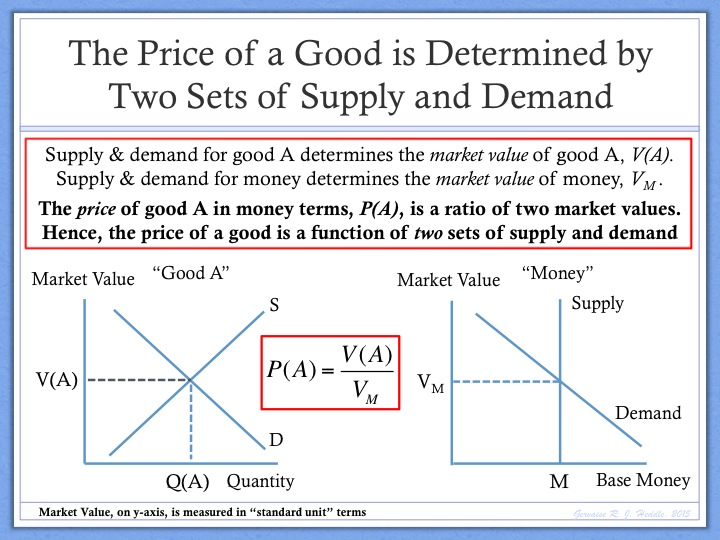
Mathematically, the price of a good in money terms is a ratio of two values (see following slide). The numerator is the market value of the good itself. The denominator is the market value of money.

The key to illustrating price determination in this way is recognizing that the property of market value can be measured in both relative and absolute terms. On the right hand side of the equation above, the market value of the good and the market value of money are both isolated as independent variables by measuring the market value of each in absolute terms. This is a rather complicated idea and I would strongly recommend that you read one of my earlier posts titled “The Measurement of Market Value: Absolute, Relative and Real” in order to more fully appreciate this concept.

This basic notion (price is a relative measurement of the market value of two goods) suggests that there are, in fact, two market processes at play in the determination of any price.

For example, in the case of the price of apples in money terms, one market process is determining the market value of apples, while another, completely different process, is determining the market value of money. The price of apples, in money terms, depends upon the equilibrium point that is found in both of these distinct processes.

Put another way, we can say that every price is a function of two sets of supply and demand. The price of one good (the primary good) in terms of another good (the measurement good) is a function of both supply and demand for the primary good and supply and demand for the measurement good.

The slide above presents the general version of this theory of price determination. Supply and demand for good A, the primary good, determines the equilibrium market value of good A. Supply and demand for good B, the measurement good, determines the equilibrium market value of good B. The price of A in B terms is determined by the ratio of these two market values. Therefore, the price of A in B terms is determined by two sets of supply and demand.

In the case of a money-based economy, the measurement good most commonly used is money. Money must possess the property of market value in order for it to be used as a medium of exchange. The view of The Money Enigma is that the market value of money is determined by supply and demand for the monetary base.

If you are interested in learning more about this microeconomic theory of price determination then I would encourage you to visit the Price Determination section of this website.

For now, the key point that matters is that the price of a good in money terms depends upon both the market value of the good itself and the market value of money. The price of a good in money terms can rise because either (1) the good itself becomes more valuable, or (2) money becomes less valuable.

If this microeconomic theory of price determination is correct, then we can extend it to the determination of the price level. After all, the price level is merely a hypothetical measure of the overall price of the basket of goods.

If every price is a relative measure of market value, then the price level is also a relative measure of market value. More specifically, the price level is a relative measure of the market value of the basket of goods in terms of the market value of money.

Rethinking the Monetary Transmission Mechanism

In simple terms, the slide above implies that the price level can rise for one of two reasons: either (1) the market value of the basket of goods rises, or (2) the market value of money falls.

While this model of price level determination may seem simplistic, it does open up an important question regarding the way in which monetary policy operates. More specifically, does an expansion of the monetary base lead to a rise in prices because (a) lower interest rates drive higher aggregate demand which leads to a rise in the market value of goods, or (b) does an increase in the monetary base somehow lead to a fall in the market value of money?

In more technical terms, does an increase in the monetary base impact the numerator (“V_G”) or the denominator (“V_M”) in our price level equation? Does it impact both? And if it does impact both, then which represents the primary monetary transmission mechanism from “more money” to “higher prices”?

We will consider the reaction of the market value of money (the denominator) to an increase in the monetary base in a moment: it is a complicated subject and we need to spend quite a bit of time thinking about it. But before we do, let’s think about how the market value of the basket of goods (the numerator) might respond to an expansion of the monetary base.

In order to assist us in this process, we are going to introduce the “Goods-Money Framework” (see slide below). In essence, the Goods-Money Framework represents an adaptation of traditional aggregate supply and demand analysis. On the left-hand side of the slide below, aggregate supply and demand determine the equilibrium market value of the basket of goods. On the right-hand side, supply and demand for money determine the market value of money. As discussed, the price is determined by the ratio of these two values.

Let’s focus on the left hand side of the slide above and think about how the equilibrium market value of goods (“V_G”) is likely to respond to an expansion in the monetary base.

The traditional Keynesian view would suggest that an expansion of the monetary base leads to a fall in interest rates. In turn, a fall in interest rates leads to an increase in aggregate demand. In terms of our slide above, the aggregate demand curve shifts to the right and the market value of the basket of goods rises. Implicitly, the Keynesian view assumes that the market value of money is constant (I say “implicitly” because Keynesian theory doesn’t recognise a role for the “value of money” in price determination). Therefore, any rise in the market value of goods is reflected as a rise in the price level.

As far as the traditional Keynesian view is concerned, this is where the story ends. An increase in money supply leads to higher demand and higher prices. The problem is that this story completely ignores the impact of lower interest rates on the aggregate supply curve.

In the real world, lower long-term interest rates not only lead to an increase in aggregate demand, but also lead to an increase in aggregate supply. In terms of our slide above, a fall in interest rates moves both aggregate demand and aggregate supply curves to the right and the impact on the equilibrium market value of goods is uncertain.

Lowering the long-term interest rate on government securities does more than just reduce mortgage rates and stimulate consumer spending: it also reduces the required return on capital for all businesses. Lowering the required return on capital stimulates expansion by existing businesses and lowers the bar to the start up of new businesses. What is the end result of all this new business activity? More supply!

When the central bank lowers the long-term interest rate by creating money and buying government securities, it effectively lowers the long-term risk free rate, a core component of the long-term required rate of return on risk assets, thereby encouraging business formation and driving an increase in aggregate supply.

Therefore, if Keynesian economists were sincere about the impact of lower interest rates, they would recognize that lower interest rates lead to both an increase in aggregate demand and aggregate supply and that the impact of monetary expansion on the absolute market value of the basket of goods is uncertain.

If this is the case, the traditional monetary transmission mechanism that is postulated by mainstream macroeconomists (more money, lower interest rates, more demand) is at best a secondary mechanism, and at worst is completely irrelevant.

Clearly, this analysis has an important implication.

If the numerator in our price level equation (the market value of the basket of goods) doesn’t act as the primary transmission mechanism from more money to higher prices, then it must be the market value of money, the denominator in our price level equation, which acts as the primary monetary transmission mechanism.

But how does “more money” impact the value of money? And if monetary base expansion should lead to a fall in the market value of money, then why have we not experienced this over the past seven years?

What Determines the Value of Money?

Those of you who are familiar with The Money Enigma will know that this is a topic that has been discussed at length over the past six months. If you want to take the crash course on this topic, then I would suggest reading “The Evolution of Money: Why Does Fiat Money Have Value?” and a follow-on post titled “What Factors Influence the Value of Fiat Money?”

For the purposes of this exercise, we will briefly discuss the nature of fiat money and how the value of fiat money is determined and then we will discuss the implications of this theory for quantity theory and the monetary transmission mechanism

The view of The Money Enigma is that fiat money is a financial instrument and derives its value solely from the nature of the liability that it represents. Fiat money is an asset to one party because it is a liability to another: fiat money is, from an economic perspective, a liability of society and represents a claim on the future output of society. More specifically, fiat money is a long-duration, special-form equity instrument and a proportional claim on the future output of society.

Every asset is either a real asset or a financial instrument. Real assets derive their value from their physical properties; financial instruments derive their value from their contractual properties.

The view of The Money Enigma is that this paradigm governs the way in which every asset, including money, derives its value. In ancient times, money was a real asset: money was a commodity (such as rice or silver) that derived its value from its physical properties.

The problem with this “commodity money” is that it restricted the ability of governments to spend (you can’t spend gold you don’t have). However, at some point, governments found a way to get around this problem: issue paper notes that promise to deliver gold on request. By issuing this first form of paper money, known as “representative money”, governments could aggressively expand their spending.

This first paper money was a financial instrument. It derived its value from its contractual properties. More specifically, it represented an explicit promise to deliver a real asset on request.

Ultimately, the issuance of representative money also limited the amount of money that governments could create. Therefore, at some point the gold convertibility feature was removed. This point marks the shift from representative money to fiat money.

In effect, the explicit contract that governed representative money was rendered null and void. So why did paper money maintain any value? The view of The Money Enigma is that the explicit contract that governed representative money was replaced by an implied-in-fact contract that governs fiat money to this day.

Fiat money is not a real asset and does not derive its value from its physical properties. Therefore, prima facie, fiat money is a financial instrument and must derive its value from its contractual properties, even if that contract is implied rather than explicit.

The exact nature of the implied-in-fact contract that governs fiat money is difficult to unravel. It is an issue that is discussed at length in the “Theory of Money” section of this website. However, in simple terms, the view of The Money Enigma is that fiat money is a liability of society and represents a claim against the future output of society.

More importantly, fiat money represents a variable entitlement to future output. In this sense, fiat money can be considered to be similar to shares of common stock: fiat money is a proportional claim on the future output of society, just as a share of common stock is a proportional claim on the future cash flow of a company

While there are important differences between the two, this concept can help us think about the factors that influence the market value of money, the denominator in our price level equation.

For example, if this theory is correct, then the value of fiat money is determined primarily by expectations regarding the long-term future path of two economic variables: real output and the monetary base.

In simple terms, future real output is the cake and the size of the future monetary base represents the number of slices the cake must be cut up into. If people become more optimistic about the long-term rate of economic growth, then the market value of money rises. Conversely, if people believe that long-term monetary base growth will be higher than previously anticipated, then the market value of money will fall.

The other important implication of this theory is that expectations regarding the long-term path of money and real output are far more important than current levels of money and real output in the determination of the value of money. Money is a long-duration asset and, like all long-duration assets, its value primarily depends on long-term expectations, not current conditions.

Why does this matter to quantity theory? Well, it may just be the missing piece that explains why quantity theory works well over long periods of time, but not short periods of time.

An Expectations-Adjusted Quantity Theory of Money

Let’s start by thinking about why the quantity theory of money works over long periods of time.

If the theory of money articulated above is correct, then for any long period of time (30 years+), an increase in the monetary base that is far in excess of the increase in real output should lead to a significant fall in the market value of money and, correspondingly, a significant rise in the price level.

If money is a proportional claim on economic output and, over a long period of time, the growth in the number of claims (the monetary base) far exceeds the growth in the economic benefit (real output), then one would reasonably expect the value of each claim to fall considerably as measured from point to point over that extended period of time.

Moreover, since the price level is a relative measure of the market value of goods in terms of the market value of money, one would also reasonably expect the price level to rise considerably over that same time period, assuming there was no reason for a massive collapse in the market value of goods.

In summary, quantity theory works in the long term because the market value of money roughly tracks the ratio of “real output/base money” over the long term.

However, the quantity theory of money breaks down over short periods of time. The reason for this is that short-term variations in the value of money are primarily driven by shifts in long-term expectations.

If you take a long hard look at the equation of exchange (the core equation of quantity theory), the one thing that should strike you about it is that it allows no explicit role for expectations in the determination of the price level.

If interpreted literally, then the equation of exchange implies that the price level is a function of only three variables: the current level of real output, the current level of money supply, and the current level of the velocity of money.

However, nearly all economists would agree that expectations play a key role in price level determination. Intuitively, it simply does not make sense to believe that prices across our economy have nothing to do with the expectations of economic agents.

So, how do we incorporate a role for expectations in the quantity theory of money?

The answer is to go back to our simple model of price level determination and think about how an increase in the quantity of money (an expansion of the monetary base) might impact both the numerator and the denominator in our price level equation.

As discussed earlier, if the numerator in our equation is relatively unresponsive to monetary policy, then it must the denominator in our equation, the market value of money that acts as the transfer agent from “more money” to “higher prices”. But we also know that “more money” (an expansion in the monetary base) does not automatically lead to a sudden fall in the value of money.

So, what are the circumstances in which an expansion of the monetary base will lead to a decline in the market value of money?

In simple terms, the rule of thumb is that an increase in the monetary base will only lead to a decline in the market value of money if that increase is believed to be “permanent” in nature. Conversely, an expansion of the monetary base will have little to no impact on the market value of money is that increase is believed to be “temporary” in nature.

Money is a long-duration asset. The value of money depends primarily not upon what is happening today, or is expected to happen in the next couple of years, but what is expected to happen over the next 20-30 years. More specifically, money is a long-duration, variable entitlement to future output. The value of money depends primarily upon expectations of the long-term path of both real output and the monetary base,.

In and of itself, a change in the current level of the monetary base is largely irrelevant to current market value of money. What really matters is how that change in the monetary base impacts expectations regarding the long-term path of the monetary base.

Putting this in the context of quantity theory, the conclusion we can draw is that it is not an increase in money supply per se that leads to an increase in the price level (although this will tend to be true when measured over long periods of time). Rather, the price level will rise if a monetary policy shift is deemed by the markets to indicate that the future growth of the monetary base will be higher than previously anticipated. Such a shift in expectations will lead to an immediate decline in the market value of money and, correspondingly, a sudden rise in the price level.

In summary, quantity theory is an important idea, but it needs to be modified to reflect the fact that expectations matter. More specifically, long-term expectations regarding the future economic prospects of society are the key determinant of the market value of money, the denominator of the price level. Moreover, it is the market value of money that acts as the primary transmission point from “too much money” to “higher prices”, whereas the interaction between monetary expansion and aggregate demand is, at best, a secondary transmission mechanism.

Author: Gervaise Heddle

Does “Too Much Money” Cause Inflation?

Does money have any role in the determination of inflation? Does printing too much money cause inflation? And what does it mean to say “too much money”? “Too much” relative to what?

Milton Friedman once famously observed, “Inflation is always and everywhere a monetary phenomenon”. Less well known is his qualification to this statement. Friedman’s full observation was “Inflation is always and everywhere a monetary phenomenon in the sense that it is and can be produced only by a more rapid increase in the quantity of money than in output.” (Friedman, “Money Mischief”, page 49)

Friedman’s qualification helps us narrow down our original question to the following, “Does too much money, relative to output, cause inflation?” Alternatively, we could ask, “Does growth in the monetary base that is significantly in excess of growth in real output cause inflation?”

Empirical evidence strongly suggests that, when measured over long periods of time, growth in the monetary base that is significantly in excess of growth in real output does lead to a concomitant rise in the price level. In this sense, Friedman’s observation appears to be correct.

However, over short periods of time, this relationship does not appear to hold. For example, over the past six or seven years, the monetary base of the United States has quadrupled, while real output has grown only modestly: yet the price level has barely moved higher.

So, why is this the case? Why does the quantity theory of money work over long periods of time, but not over short periods of time?

The view of The Money Enigma is that, over short periods of time, the primary driver of inflation is not the change in the current ratio of “base money/real output”, but the change in the expected 20-30 year future ratio of “base money/real output”. In other words, it is not the current level of growth in money relative to output that matters, but rather the expected long-term future growth of money relative to output that matters.

In this sense, it is not “too much money” that causes inflation, but the expectation of “too much money” being created over the next 20 years that matters.

Why might market participants suddenly expect a society to create too much money (relative to output) in the future? There are many possible reasons, but obvious reasons might include war, a secular decline in productivity, economic mismanagement, or just the sudden realization that a country has been living way beyond it means.

Inflation and the value of money

In the academic world, fashions come and go. In the late 1960s and early 1970s, there was much discussion about the role of money in the determination of inflation, a discussion that was led by the great minds of that time including Milton Friedman, Anna Schwartz and Philip Cagan.

Fast forward nearly fifty years, and it is not fashionable to discuss the role of money in the determination of the price level. Indeed, there is a view among many economists (notably, New Keynesian economists) that money is almost irrelevant to the discussion and that the size of the monetary base is only important in so far as it influences interest rates.

This is despite the fact that one of the strongest empirical relationships in economics remains the long-term correlation between the price level and the ratio of base money to real output. As Friedman once put it, inflation “…is and can be produced only by a more rapid increase in the quantity of money than in output.” This sentiment is clearly supported by the long-term data.

So, why is there such a disconnect? Why do academic economists largely dismiss the important role that the money/output ratio has in the determination of inflation?

First, the correlation between the price level and the money/output ratio breaks down in the short term. Although the quantity theory of money is valid over very long periods of time, it doesn’t work over short periods of time. Therefore, most economists feel comfortable ignoring quantity theory in their short-term forecasting of inflation.

Second, mainstream economics does not recognize the important role that the value of money plays in the determination of the price level. According to the orthodox view, the “value of money” has nothing to do with price determination!

Indeed, mainstream economics does not officially recognise the “market value of money” as a variable in any of its equations. Mainstream economics does not recognise the “market value of money” as a relevant economic variable because the view of mainstream (Keynesian) economics is that supply and demand for money determines the interest rate.

The view of The Money Enigma is that supply and demand for money (the monetary base) determines the market value of money (not the interest rate). In turn, the market value of money is the denominator of every money price in the economy and, therefore, is the denominator of the price level.

This general issue was discussed in a recent post titled “The Interest Rate is Not the Price of Money“. But rather than dwell on Keynesian theory, let’s briefly discuss how prices are determined at both a micro and macro level and then use this to continue with our discussion of the relationship between money and inflation.

What is a “price” and how is a price determined?

Price determination is a subject that we have discussed extensively over the past few months, so I don’t want to dwell on it in this post. We will discuss the basic principles today, but if you want more detail you should read the following posts:

“Every Price is a Function of Two Sets of Supply and Demand” (01/20/15)

“The Measurement of Market Value: Absolute, Relative and Real” (04/21/15)

“A New Economic Theory of Price Determination” (04/28/15)

In simple terms, the view of The Money Enigma is that every price is a relative expression of the market value of two goods.

Consider a simple exchange of two goods. Both goods must possess the property of market value in order for them to be exchanged. The price of the exchange simply measures the market value of one good in terms of another: the market value of a “primary good” in terms of the market value of a “measurement good”.

In our modern money-based economy, the measurement good most commonly used is money. The price of a good, in money terms, simply reflects the market value of the good relative to the market value of money. For example, if the price of a banana is $2, then we can say that the market value of one banana is twice the market value of one dollar.

The key point is that the price of a banana, in money terms, is a relative measure of value: it is determined not just by the market value of the banana (which can rise and fall) but also the market value of money (which can also rise and fall). If the market value of money falls, then, all else remaining equal, the price of the banana in money terms will rise.

In this sense, the market value of money is the denominator of every “money price” in the economy. In mathematical terms, the price of a good, in money terms, is a ratio of the market value of the good divided by the market value of money.

The trick to expressing this in terms of mathematical formula is recognizing that market value can be measured in the absolute. Just as we can measure any physical property in the absolute by using a “standard unit” of measurement for that property, so market value can be measured in the absolute by using a “standard unit” of measurement for market value.

The height of a tree can be measured using a standard unit for the measurement of height, namely “inches”. An “inch” is an invariable measure of the property of height. In economics, we can create an invariable measure of market value: a standard unit” for the measurement of market value that possesses the property of market value and is invariable in this property. Since no good exists that is invariable in market value, we need to create a theoretical measure, called “units of economic value”.

Once we have a standard unit for the measurement of market value, we can measure the market value of both goods being exchanged in terms of this standard unit. In other words, we can measure the market value of both goods in absolute terms.

This raises an obvious question: how is the market value of a good determined? In this respect, we can adapt an old paradigm: the market value of a good is determined by supply and demand for that good. If we plot supply and demand for each good in terms of our standard unit of market value, then we can see that the price of the primary good (good A) in terms of the measurement good (good B) is a function of two sets of supply and demand.

Supply and demand for the primary good (good A) determines the market value of the primary good. Supply and demand for the measurement good (good B) determines the market value of the measurement good. The price of the primary good in terms of the measurement good (the price of A in B terms) is the ratio of the market value of the primary good divided by the market value of the measurement good. This is a universal theory of price determination that we can apply to the determination of barter prices (good/good prices), money prices (good/money prices) and foreign exchange rates (money/money prices).

In a money-based economy, the price of a good, in money terms, is determined by the ratio of the market value of the good divided by the market value of money.

We can extend this microeconomic principle to a macroeconomic description of price level determination. If the market value of money is the denominator of every “money price” in our economy, then the market value of money is the denominator of the price level. (Remember, the price level is nothing more than a hypothetical measure of overall money prices for the set of goods and services that comprise the “basket of goods”.)

Once again, if we measure the overall market value of goods and services in terms of a standard unit of market value and denote this as V_G, and we measure the market value of money in terms of the same standard unit and denote this as V_M, then the price level is simply a ratio of V_G and V_M.

Ratio Theory of the Price Level simply states that the price level depends upon both the overall market value of the basket of goods and services and the market value of money. If the market value of the basket of goods and services is relatively stable over time, then the price level will be primarily determined by the direction of the market value of money. If the market value of money falls significantly over time, then the price level will rise significantly over that same period of time.

The determination of the market value of money

The view of The Money Enigma is that the market value of money is the denominator of every “money price” in the economy: the price of a good, in money terms, depends upon both the market value of the good and the market value of money.

If this theory is correct, then the market value of money plays a critical role in the determination of the price level and inflation. So, what determines the market value of money?

We have already hinted at part of the answer: supply and demand.

If every price is a function of two sets of supply and demand, then every money price must be a function of two sets of supply and demand. More specifically, the price of good A, in money terms, depends upon both supply and demand for good A and supply and demand for money (the monetary base).

As discussed in the introduction, the view of The Money Enigma is that supply and demand for money (the monetary base) determines the market value of money, not the interest rate. (The interest rate is determined by supply and demand for loanable funds).

While this might be an interesting first step, it really doesn’t tell us much about the factors that influence the value of money. In order to understand the specific factors that determine the market value of money, we need to develop a deeper understanding of what money is.

Over the past two weeks, we have discussed the nature of fiat money at length. In the first post, “The Evolution of Money: Why Does Fiat Money Have Value?” we traced the evolution of money from “commodity money” to “representative money” and finally to “fiat money”.

In that post, it was argued that representative money derives its value from an explicit contract: representative money is just a piece of paper that promises the holder of that piece of paper a real asset (normally, gold or silver) when that piece of paper is presented to its issuer.

When the gold/silver convertibility feature was removed, i.e. when the explicit contract was rendered null and void and the representative money became fiat money, the explicit contract was replaced by an implied-in-fact contract. In this way, fiat money derives its value contractually. Every asset derives its value from its physical properties (it is a real asset) or from its contractual properties (it is a financial instrument). Fiat money is not a real asset. Therefore, fiat money must be a financial instrument that derives its value from its contractual features.

The nature of the implied contract that governs fiat money was explored in a second post, “What Factors Influence the Value of Fiat Money?” While it is difficult to speculate on the exact nature of the implied contract, we can leverage finance theory to guide us in the right direction.

The view of The Money Enigma is that fiat money is a special-form, long-duration equity instrument issued by society. More specifically, fiat money represents a proportional claim on the future output of society.

And this brings us to the crux of the issue: what determines the value of fiat money and, consequently, the level of money prices in the economy?

If money is a proportional claim on the future output of society, then its value depends, at least primarily, upon future expectations of (1) real output, and (2) the size of the monetary base. Moreover, if money is a long-duration asset, then its value depends upon expectations regarding the long-term (20-30 year) path of these two important variables (real output and base money).

If the market suddenly decides that long-term (20 year) real output growth will be higher than previously anticipated, then the value of a proportional claim on that future output should rise (the market value of money should rise). All else remaining equal, the value of money will rise and the price level will fall.

In this example, there has been no change in current levels of real output or the monetary base, yet the price level has fallen. Why? The price level falls because it depends on the market value of money (the market value of money is the denominator of the price as per “Ratio Theory”). In turn, the market value of money depends upon long-term expectations. Current conditions really only matter to the market value of money to the degree that they impact expectations of long-term conditions. This is true of the value of any long-duration asset: current conditions are only important to the value of a long-duration asset in so far as they impact long-term expectations.

Now, let’s consider what happens if the market suddenly decides that the long-term growth rate of the monetary base will be much higher than previously anticipated. If money is a proportional claim on output, then more claims at some future point will mean that every claim is entitled to a smaller proportionate share of output at that future point. If the market decides that the future value of money will be lower, then this will have an immediate negative impact on the current value of money. Why? In simple terms, the market value of money depends upon a chain of future expectations regarding the future value of money.

Admittedly, this is a complicated concept and one that is explored in much greater detail in The Velocity Enigma, the third and final paper of The Enigma Series.

The key point that I wish to highlight is that, if proportional claim theory is correct, then the current market value of money depends upon the expected long-term path of both real output and the monetary base. Furthermore, since the market value of money is the denominator of the price level, the price level itself also depends upon the expected long-term path of both real output and the monetary base.

Bearing this in my mind, let’s return to our original question.

Does “too much money” cause inflation?

There can be little doubt that, over long periods of time (30 years+), growth in the monetary base that is greatly in excess of growth in real output will lead to a rise in the price level. There is strong empirical support for this observation.

This observation sits neatly with the theory that money is a proportional claim on the output of society. Over long periods of time, if the number of claims on output grows at a substantially faster rate than output, then the value of each claim should fall. In other words, if the monetary base grows at a substantially faster rate than output, then the market value of money should fall and the price level should rise (the market value of money is the denominator of the price level).

On the other hand, there is also compelling evidence to indicate that, over short periods of time, a dramatic increase in the monetary base can have little to no impact on the market value of money, even if the increase in the monetary base dwarfs any increase in real output during that same period of time.

This phenomenon has always been harder for economists to explain, but it can be explained by the theory that money is a special-form equity instrument and a long-duration, proportional claim on the future output of society.

If money is a long-duration, proportional claim on output, then the value of money will only be sensitive to changes in current levels of real output and the monetary base to the degree that changes in current levels impact expectations regarding the long-term path of both real output and the monetary base.

We can use a simple analogy from finance: the value of shares. The value of a share of common stock depends on the expected future cash flows that will accrue to the holder of that share. More specifically, a company’s stock price depends little on current earnings or current shares outstanding. Rather, the stock price is determined by expected long-term earnings per share. Therefore, it is the long-term path of both net earnings and shares outstanding that matter to the current value of a share of common stock.

Similarly, money is a long-duration asset and its value is primarily driven by expectations of the long-term real output/base money ratio, not by the current real output/base money ratio.

This has one important implication regarding market perception of monetary policy and its impact on inflation. If the market believes that a sudden rise in the monetary base is only “temporary” (it will be reversed in the next few years), then such an increase in the monetary base should have little to no impact on the value of money and, therefore, little to no impact on the price level.

However, if the market believes that a sudden rise in the monetary base is more “permanent” in nature, then that increase in the monetary base should lead to a fall in the value of money and a rise in the price level.

The view of The Money Enigma is that the dramatic increase in the monetary base in the United States has had little impact on the market value of the US Dollar (and little impact on the price level) because market participants believe that the increase is “temporary” in nature.

In slightly more sophisticated terms, the extraordinary actions of the Fed have not changed the market’s view regarding the long-term (20-30 year) path of the real output/base money ratio. Most market participants remain optimistic that real output will grow at solid rates for he next 30 years, even while the monetary base is reduced or at least capped at current levels. This has put a floor under the value of the US Dollar and a lid on the price level.

However, what happens if market expectations change? What will happen if the market becomes more pessimistic regarding the long-term economic prospects of the United States?

If market participants begin to believe that the Fed is unwilling or unable to reduce the monetary base, then this shift in expectations will begin to put downward pressure on the value of money and upward pressure on the price level. This fall in the value of money will be compounded if the market becomes more pessimistic about the long-term rate of real output growth in the United States. If this were to occur, then a return to double-digit levels of inflation is quite possible.

What Causes Inflation?

Inflation remains one of the great enigmas of modern economics. In this week’s post, we will examine a simple theory of the price level, “Ratio Theory of the Price Level”, and a basic model that can be used for thinking about short-term movements in the price level “The Goods-Money Framework”. We will then use these ideas to examine some of the traditional explanations for inflation.

Despite extensive academic studies and seemingly endless debate, a quick keyword search on “what causes inflation?” will reveal a jungle of different ideas and opinions regarding the true drivers of inflation.

The traditional view, taught at high schools and colleges, is that inflation can be driven by “demand pull” or “cost push” factors. In essence, this is a macroeconomic extension of the basic microeconomic tenet that the price of a good can rise either because there is more demand for that good (“demand pull”) or because there is reduced supply for that good (“cost push”).

The “demand pull/cost push” model represents an “old Keynesian” view of how the world works: if aggregate demand increases, then real output should increase and the price level will rise, particularly if the economy is operating near full capacity.

Mainstream economists recognize that this simple aggregate supply and demand view of the world often fails to predict episodes of high inflation. Therefore, this basic Keynesian model has been fudged by the addition of something called “inflation expectations”. This “New Keynesian” model states that inflation is caused by either (1) too much demand, or (2) expectations of future inflation. The problem with the “inflation expectations” term in the New Keynesian models is that no one seems to have a good sense of what determines “inflation expectations”.

The issue is made more complicated by the fact that most economists recognize that, over the long term, the monetary base plays an important role in the determination of the price level. Even senior central bankers tie themselves in knots trying to explain how to reconcile the New Keynesian model of the world with the simple, empirical fact that money matters. Mervyn King, former Governor of the Bank of England, discusses this problem in his article “No money, no inflation – the role of money in the economy” (2002) in which he concludes that “the absence of money in the standard models which economists use will cause problems in the future”. Frankly, I couldn’t agree more.

If even central bankers can’t reconcile the competing views of what drives inflation, then this suggests that something is wrong with the underlying models. The view of The Money Enigma is that both Keynesian and Monetarist models fail to provide satisfactory models for the determination of the price level because they both start from the wrong fundamentals.

In order to build useful models of the price level, we need to go back and challenge the basics of current microeconomic theory. In particular, we need to develop a more comprehensive answer to the question “how is a price determined?”

It is the view of The Enigma Series that the current presentation of microeconomic price determination, namely the traditional supply and demand chart with price on the y-axis, presents a one-sided and very limited view of the price determination process.

The view of The Enigma Series is that every price is a function of two sets of supply and demand. More specifically, the price of one good (the primary good) in terms of another good (the measurement good) is a function of both supply and demand for the primary good and supply and demand for the measurement good.

A few weeks ago, we discussed how prices are determined in a genuine barter economy (an economy in which there is no commonly accepted medium of exchange). We asked the question “what determines the price of apples in banana terms? Is it supply and demand for apples? Or is it supply and demand for bananas?” The answer is both.

Every price is a relative expression of two market values. The market value of apples is determined by supply and demand for apples. The market value of bananas is determined by supply and demand for bananas. The price of apples, in banana terms, is a relative expression (a ratio) of these two market values. Therefore, the price of apples, in banana terms, is a function of two sets of supply and demand (see diagram below).

This principle can be extended to the determination of “money prices”. The price of a good, in money terms, is a relative expression of the market value of the good and the market value of money. For example, if the market value of one apple is three times the market value of one US Dollar, then the price of an apple, in US Dollar terms, is three dollars.

In general terms, the dollar price of an apple can rise for one of two reasons: either the market value of an apple rises (for example, there is a supply shortage), or the market value of the dollar falls.

The diagram below illustrates how the price of apples, in money terms, is determined by two sets of supply and demand: supply and demand for apples, and supply and demand for money. The key in this diagram is the y-axis unit of measurement: a “standard unit” of market value. Instead of using price, a relative measure of market value, on the y-axis, the diagrams above and below use an absolute measure of market value of the y-axis. The standard unit of market value is a theoretical and invariable measure of the property of market value, just as “inches” are an invariable measure of the property of length.

The key point that readers should take away from the above diagram is that every “money price” in our economy is a ratio. More specifically, the price of a good in money terms is a ratio of the market value of the good (the numerator) divided by the market value of money (the denominator).

The Inflation Enigma, the second paper in The Enigma Series, extends this simple microeconomic concept (every price is a relative expression of two market values) to a macroeconomic level. If the market value of money is the denominator of every money price in the economy, then the price level can be stated as a ratio of two market values: the “general value level”, a hypothetical measure of the absolute market value of the basket of goods/services, and the market value of money. This is called the Ratio Theory of the Price Level.

Ratio Theory of the Price Level states that the price level is a function of the value of goods relative to the value of money. If the value of goods rises relative to the value of money, then the price level rises (inflation). If the value of goods falls relative to the value of money, the price level falls (deflation).

We can best illustrate Ratio Theory with a simple macroeconomic framework called “The Goods-Money Framework” (see diagram below). The Goods-Money Framework is broken into a left side and right side. On the left side, aggregate supply and demand for goods/services determines real output (x-axis) and the market value of goods (y-axis), as measured in absolute terms. On the right side, supply and demand for money (the monetary base) determines the market value of money (again, market value is measured in absolute terms).

The price level is a ratio of two macroeconomic equilibrium: the market value of goods, as determined on the left side of the model, divided by the market value of money, as determined on the right side of the model. Now, let’s get back to our original question.

What causes inflation?

The left side of the Goods-Money Framework provides some distinctly Keynesian answers to this question. All else equal, the price level will rise if the market value of goods (the “general value level”) rises. In a stylized sense, this can occur either because the aggregate demand curve shifts to the right (“demand pull”) or because the aggregate supply curve shifts to the left (“cost push”).

The right side of the Goods-Money Framework provides a somewhat more Monetarist perspective on the issue. All else equal, the price level will rise is the market value of money falls. In very simple terms, this can occur either because the supply of money (the monetary base) increases or because the demand for money falls.

In practice, both the left side and right side of the model are both moving at the same time. For example, deflationary forces that are acting on the left side of the model, (for example, “globalization” of the labor force), might be offset by inflationary forces on the right side (for example, aggressive monetary easing), leading to a net result where the price level changes little. [Note: if both the numerator and denominator fall by roughly the same percentage, then there is no change to the ratio itself].

While interpreting the left side of the framework is relatively straightforward, the right side of the framework is extremely complex. The main problem is that “supply and demand” is, in practice, a poor short-term model for the determination of the market value of money.

We know from recent experience that a large increase in the monetary base can have little short-term impact on the market value of money (and hence, little short-term impact on the price level). The reason for this is that money is a proportional claim on the future output of society. More importantly, money is a long-duration asset. The market value of money depends far more upon expectations of future levels of the monetary base than it does on the current levels of the monetary base.

The Velocity Enigma, the final paper in The Enigma Series, develops a valuation model for money that demonstrates that the current market value of money depends upon long-term expectations. More specifically, the current market value of money is highly dependent upon the expected long-term path of the “real output/base money” ratio.

As you can see, there is no simple answer to the question “what causes inflation?”

The traditional Keynesian view provides a very limited perspective on the issue. Importantly, the notion that inflation can only occur if the economy is overheating (the economy can only experience inflation if there is “too much demand”) is nonsense.

The price level depends upon a complex set of expectations. Most notably, the expected long-term path of the “real output/base money” ratio is the key determinant of the market value of money. In turn, the market value of money is the denominator of every “money price” in the economy.

This model provides a sensible explanation for how inflation can occur in a weak economic environment. If aggregate demand is weak, then this will place downward pressure on the market value of goods on the left side of our model. However, if confidence in the economic future of the country falters, then this can easily lead to a decline in the market value of money that overwhelms the fall in the market value of goods. In the context of Ratio Theory, as the denominator (the market value of money) falls more rapidly than the numerator (the market value of goods), the price level rises.

In summary, we can say that, in the short-term, the drivers of the price level are complex. Aggregate demand and supply matter, but expectations of the future path of the “real output/base money” ratio are critical.

While economists may disagree on the short-term drivers of the price level, there is at least a broader consensus on what drives the price level over the long-term: money. More specifically, the ratio of base money to real output is the key driver of the price level as measured from point to point over very long periods of time.

The Enigma Series provides a common sense explanation for this phenomenon.

Money is a special-form equity instrument of society that represents a proportional claim on the future output of society. The value of a proportional claim on the output of society will rise as real output rises and fall as the monetary base increases (i.e. as the number of claims against that output increases).

Therefore, if over a period of many years, the monetary base has grown at a much faster rate than real output (as it has in the United States over the past 80 years), we should expect the market value of money to have fallen significantly and, all else equal, the price level should have risen significantly.

Over long periods of time, it is this ratio of money/output that drives the price level. The question today is how long can the monetary base in the United States can remain at these extended levels without triggering a significant decline in the market value of money and reigniting inflation. Too many commentators who are worried about deflation are, at least implicitly, focused only on the left side of our model above. The key to inflation remains the right side of the model, the market value of money.

Share this:

Share this:

Share this:

Share this: